原文:https://gafferongames.com/post/fix_your_timestep/

這篇文章主要說了：怎么正確的實現一個 固定時常的Tick方式，有些類似于unity的 fixedupdate的實現。

實現方式：1.時間的累計，并且一幀可能會執行多次 fixedTick  2.針對Render渲染幀，進行時間的插值，確保和fixedTick里的邏輯同步。

比較適合在fixedTick里實現的邏輯。最常見的是物理模擬。

我只翻譯兩部分：

Semi-fixed timestep  半固定時間步長

It’s much more realistic to say that your simulation is well behaved only if delta time is less than or equal to some maximum value. This is usually significantly easier in practice than attempting to make your simulation bulletproof at a wide range of delta time values.

With this knowledge at hand, here’s a simple trick to ensure that you never pass in a delta time greater than the maximum value, while still running at the correct speed on different machines:

  double t = 0.0;
    double dt = 1 / 60.0;

    double currentTime = hires_time_in_seconds();

    while ( !quit )
    {
        double newTime = hires_time_in_seconds();
        double frameTime = newTime - currentTime;
        currentTime = newTime;
              
        while ( frameTime > 0.0 )
        {
            float deltaTime = min( frameTime, dt );
            integrate( state, t, deltaTime );
            frameTime -= deltaTime;
            t += deltaTime;
        }

        render( state );
    }

The benefit of this approach is that we now have an upper bound on delta time. It’s never larger than this value because if it is we subdivide the timestep. The disadvantage is that we’re now taking multiple steps per-display update including one additional step to consume any the remainder of frame time not divisible by dt. This is no problem if you are render bound, but if your simulation is the most expensive part of your frame you could run into the so called “spiral of death”.

What is the spiral of death? It’s what happens when your physics simulation can’t keep up with the steps it’s asked to take. For example, if your simulation is told: “OK, please simulate X seconds worth of physics” and if it takes Y seconds of real time to do so where Y > X, then it doesn’t take Einstein to realize that over time your simulation falls behind. It’s called the spiral of death because being behind causes your update to simulate more steps to catch up, which causes you to fall further behind, which causes you to simulate more steps…

如果你的物理模擬無法跟上所需的計算步數，你的程序就會陷入一個惡性循環。例如：

1. 你的游戲需要模擬 X 秒的物理。
2. 但物理計算需要 Y 秒（Y > X）。
3. 由于 Y > X，你的模擬會逐漸落后。
4. 為了追趕進度，模擬需要執行更多的步驟……
5. 但這又導致它變得更慢，最終進入無限循環。

So how do we avoid this? In order to ensure a stable update I recommend leaving some headroom. You really need to ensure that it takes significantly less than X seconds of real time to update X seconds worth of physics simulation. If you can do this then your physics engine can “catch up” from any temporary spike by simulating more frames. Alternatively you can clamp at a maximum # of steps per-frame and the simulation will appear to slow down under heavy load. Arguably this is better than spiraling to death, especially if the heavy load is just a temporary spike.

Free the physics 解耦物理更新和渲染

Now let’s take it one step further. What if you want exact reproducibility from one run to the next given the same inputs? This comes in handy when trying to network your physics simulation using deterministic lockstep, but it’s also generally a nice thing to know that your simulation behaves exactly the same from one run to the next without any potential for different behavior depending on the render framerate.

為了確保物理模擬在相同輸入下，每次運行的結果都完全一致，我們需要采用完全固定的時間步長，你的模擬從一次運行到下一次運行的行為完全相同而沒有任何可能因渲染幀率而不同的行為也是件好事。

But you ask why is it necessary to have fully fixed delta time to do this? Surely the semi-fixed delta time with the small remainder step is “good enough”? And yes, you are right. It is good enough in most cases but it is not exactly the same due to to the limited precision of floating point arithmetic.

但是你會問為什么需要完全固定的時間來做這個？半固定的時間和小的剩余步長肯定是“足夠好”嗎？是的，你是對的。在大多數情況下，它已經足夠好了，但由于浮點運算的精度有限，它并不完全相同。

What we want then is the best of both worlds: a fixed delta time value for the simulation plus the ability to render at different framerates. These two things seem completely at odds, and they are - unless we can find a way to decouple the simulation and rendering framerates.

解耦simulation幀和render幀

Here’s how to do it. Advance the physics simulation ahead in fixed dt time steps while also making sure that it keeps up with the timer values coming from the renderer so that the simulation advances at the correct rate. For example, if the display framerate is 50fps and the simulation runs at 100fps then we need to take two physics steps every display update. Easy.

What if the display framerate is 200fps? Well in this case it we need to take half a physics step each display update, but we can’t do that, we must advance with constant dt. So we take one physics step every two display updates.

Even trickier, what if the display framerate is 60fps, but we want our simulation to run at 100fps? There is no easy multiple. What if VSYNC is disabled and the display frame rate fluctuates from frame to frame?

If you head just exploded don’t worry, all that is needed to solve this is to change your point of view. Instead of thinking that you have a certain amount of frame time you must simulate before rendering, flip your viewpoint upside down and think of it like this: the renderer produces time and the simulation consumes it in discrete dt sized steps.

Notice that unlike the semi-fixed timestep we only ever integrate with steps sized dt so it follows that in the common case we have some unsimulated time left over at the end of each frame. This left over time is passed on to the next frame via the accumulator variable and is not thrown away.

注意，與半固定時間步長不同的是，我們只對步長dt進行積分，因此，在一般情況下，在每一幀結束時，我們會留下一些未模擬的時間。剩余的時間通過累加器變量傳遞到下一幀，不會被丟棄。

The final touch

But what do to with this remaining time? It seems incorrect doesn’t it?

To understand what is going on consider a situation where the display framerate is 60fps and the physics is running at 50fps. There is no nice multiple so the accumulator causes the simulation to alternate between mostly taking one and occasionally two physics steps per-frame when the remainders “accumulate” above dt.

Now consider that the majority of render frames will have some small remainder of frame time left in the accumulator that cannot be simulated because it is less than dt. This means we’re displaying the state of the physics simulation at a time slightly different from the render time, causing a subtle but visually unpleasant stuttering of the physics simulation on the screen.

One solution to this problem is to interpolate between the previous and current physics state based on how much time is left in the accumulator:

    double t = 0.0;
    double dt = 0.01;

    double currentTime = hires_time_in_seconds();
    double accumulator = 0.0;

    State previous;
    State current;

    while ( !quit )
    {
        double newTime = time();
        double frameTime = newTime - currentTime;
        if ( frameTime > 0.25 )
            frameTime = 0.25;
        currentTime = newTime;

        accumulator += frameTime;

        while ( accumulator >= dt )
        {
            previousState = currentState;
            integrate( currentState, t, dt );
            t += dt;
            accumulator -= dt;
        }

        const double alpha = accumulator / dt;

        State state = currentState * alpha + 
            previousState * ( 1.0 - alpha );

        render( state );
    }

This looks complicated but here is a simple way to think about it. Any remainder in the accumulator is effectively a measure of just how much more time is required before another whole physics step can be taken. For example, a remainder of dt/2 means that we are currently halfway between the current physics step and the next. A remainder of dt*0.1 means that the update is 1/10th of the way between the current and the next state.

We can use this remainder value to get a blending factor between the previous and current physics state simply by dividing by dt. This gives an alpha value in the range [0,1] which is used to perform a linear interpolation between the two physics states to get the current state to render. This interpolation is easy to do for single values and for vector state values. You can even use it with full 3D rigid body dynamics if you store your orientation as a quaternion and use a spherical linear interpolation (slerp) to blend between the previous and current orientations.

https://docs.unity3d.com/6000.0/Documentation/Manual/fixed-updates.html

我們看untity文檔里對于FixedUpdate的描述，基本和上面的實現類似。

The fixed update loop simulates code running at fixed time intervals but in practice the interval between fixed updates isn’t fixed. This is because a fixed update always needs a frame to run in and the duration of a frame and the length of the fixed time step are not in perfect sync. If a fixed time step completes during the current frame, the associated fixed update can’t run until the next frame. When frame rates are low, a single frame might span several fixed time steps. In this case a backlog of fixed updates accumulates during the current frame and Unity executes all of them in the next frame to catch up.

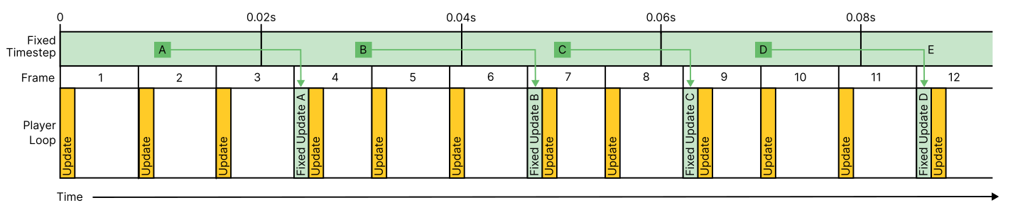
An example showing FixedUpdate running at 50 updates per second (0.02s per fixed update) and the Player Loop running at approximately 80 frames per second. Some frame updates (marked in yellow) have a corresponding FixedUpdate (marked in green) if a new complete fixed timestep has elapsed by the start of the frame.

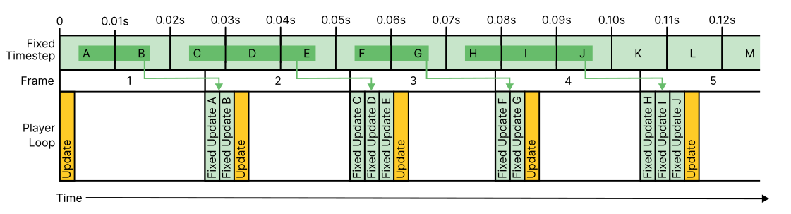
 An example showing Update running at 25 FPS and FixedUpdate running at 100 updates per second. You can see there are four occurrences of a FixedUpdate during one frame, marked in yellow.

Note: A lower timestep value means more frequent physics updates and more precise simulations, which leads to higher CPU load.

低幀率情況下，fixedupdate執行頻率變高，CPU壓力變得更大了。。

也就是說 如果設備由于各種Profile原因導致FPS變低，如果一直保持一個很低的水平，導致FixedUpdated同一幀執行次數變多，那CPU就會更低了。。