一文讀懂什么是邏輯回歸
邏輯回歸介紹

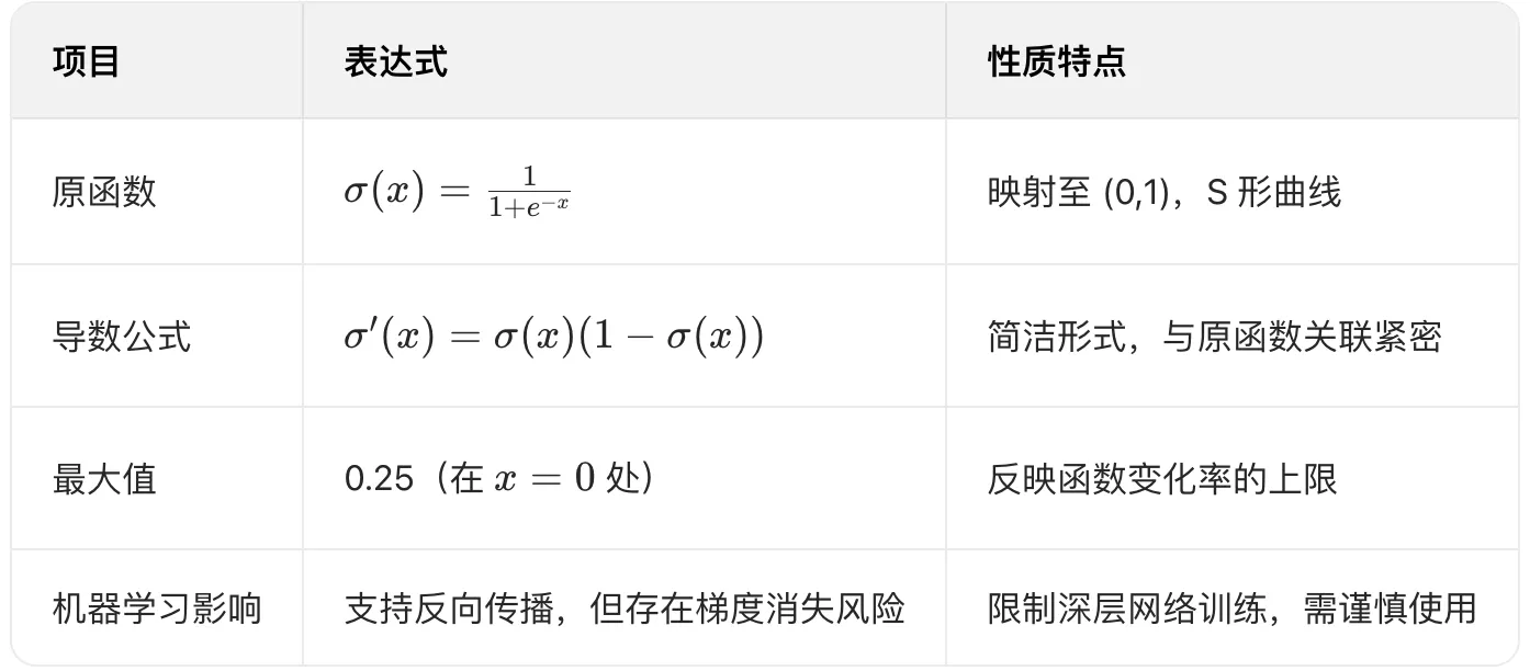
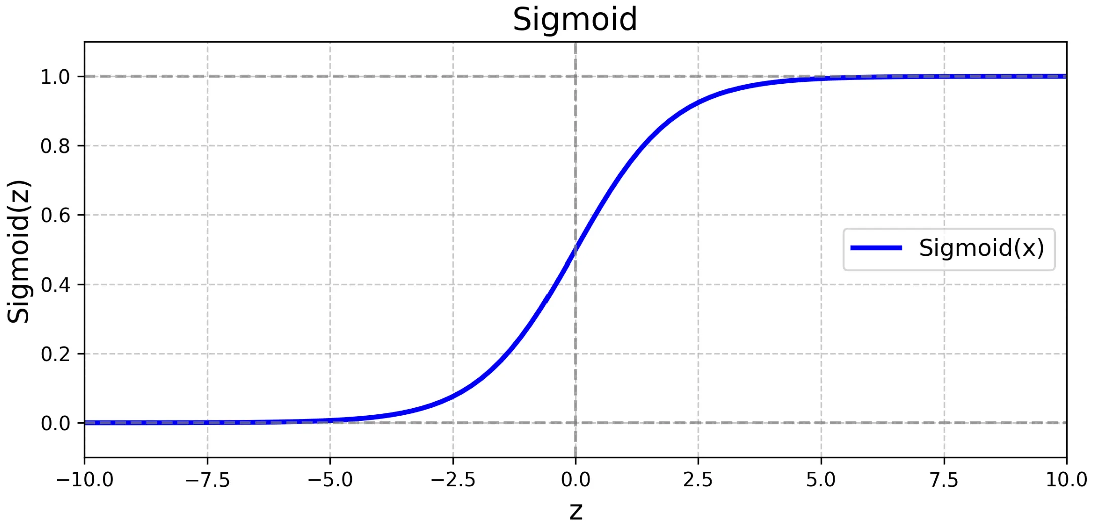
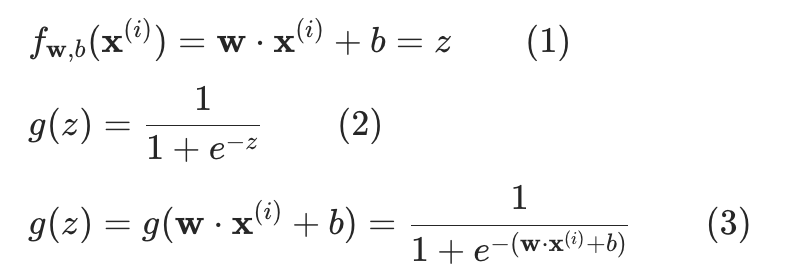
sigmoid函數
def sigmoid(z):
    """
    Compute the sigmoid of z

    Args:
        z (ndarray): A scalar, numpy array of any size.

    Returns:
        g (ndarray): sigmoid(z), with the same shape as z

    """

    g = 1 / (1 + np.exp(-z))

    return g
邏輯回歸模型
邏輯回歸的決策邊界
線性邏輯回歸
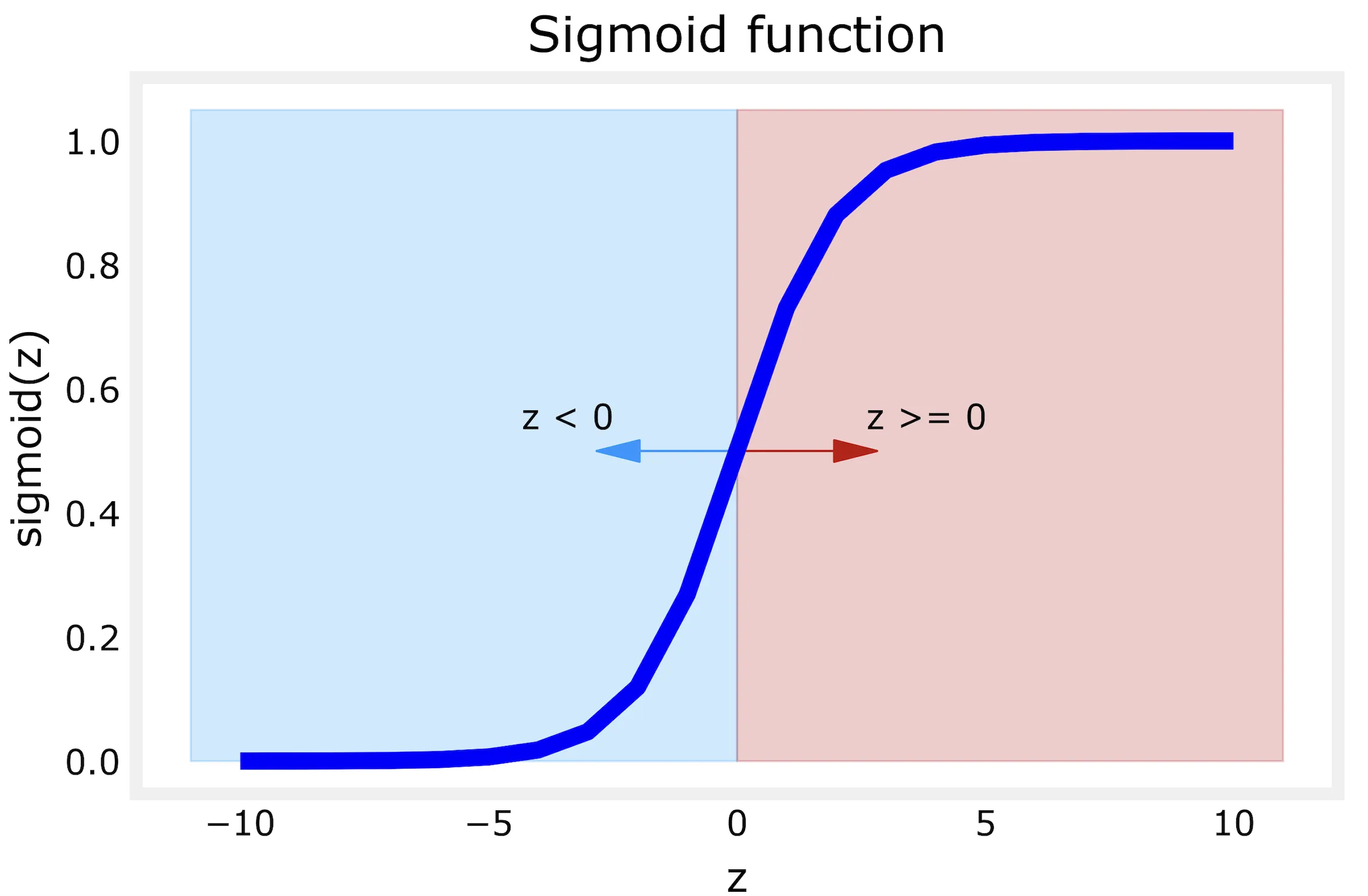
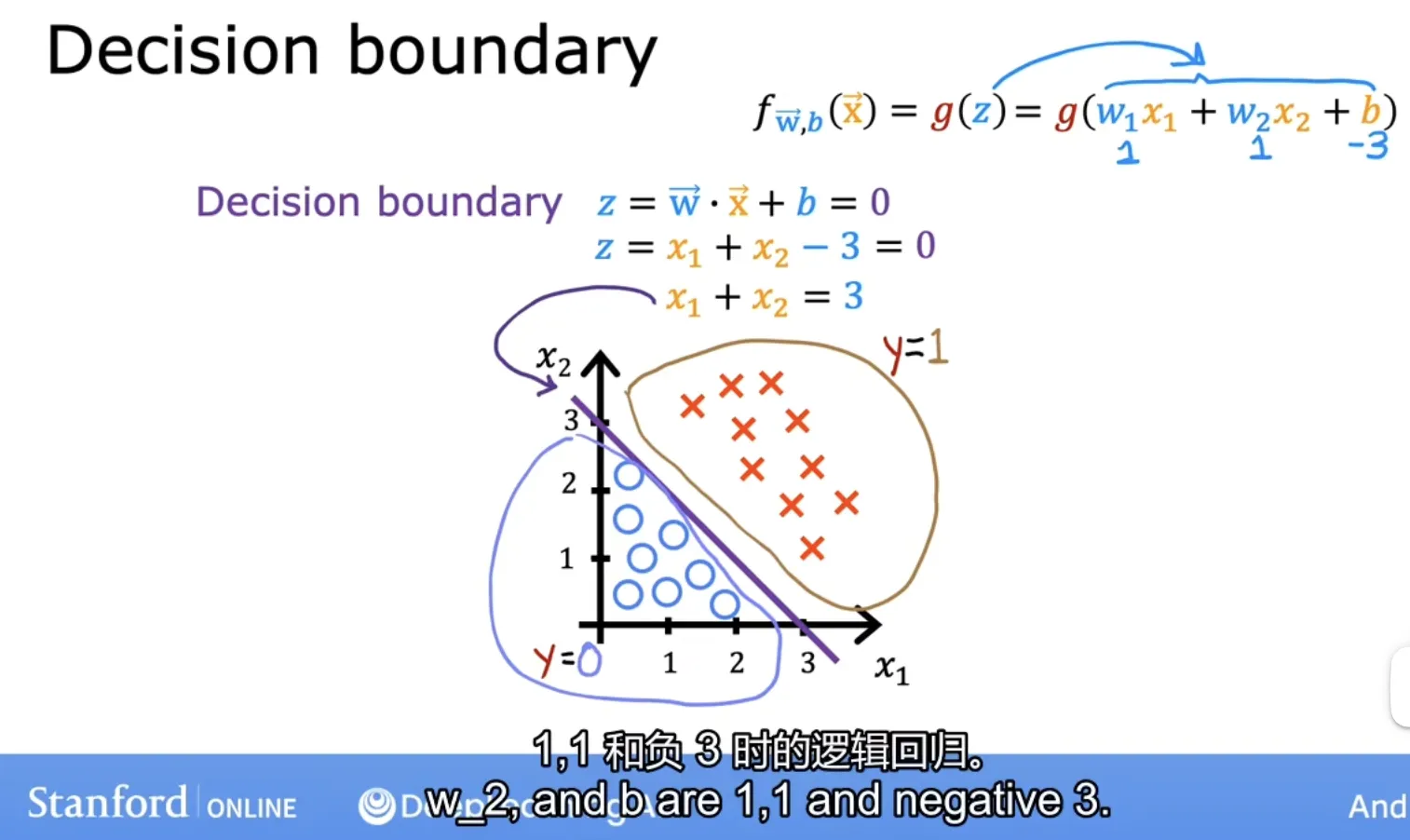
根據sigmoid函數圖象:z=0是中間位置,視為決策邊界;那么為了得到決策邊界的特征情況,我們假設:
- 線性模型
z = w1 * x1 + w2 * x2 + b - 參數
w1=w2=1, b=03,那么x2 = -x1 + 3這條直線就是決策邊界
如果特征x在這條線的右邊,那么此邏輯回歸則預測為1,反之則預測為0;(分為兩類)
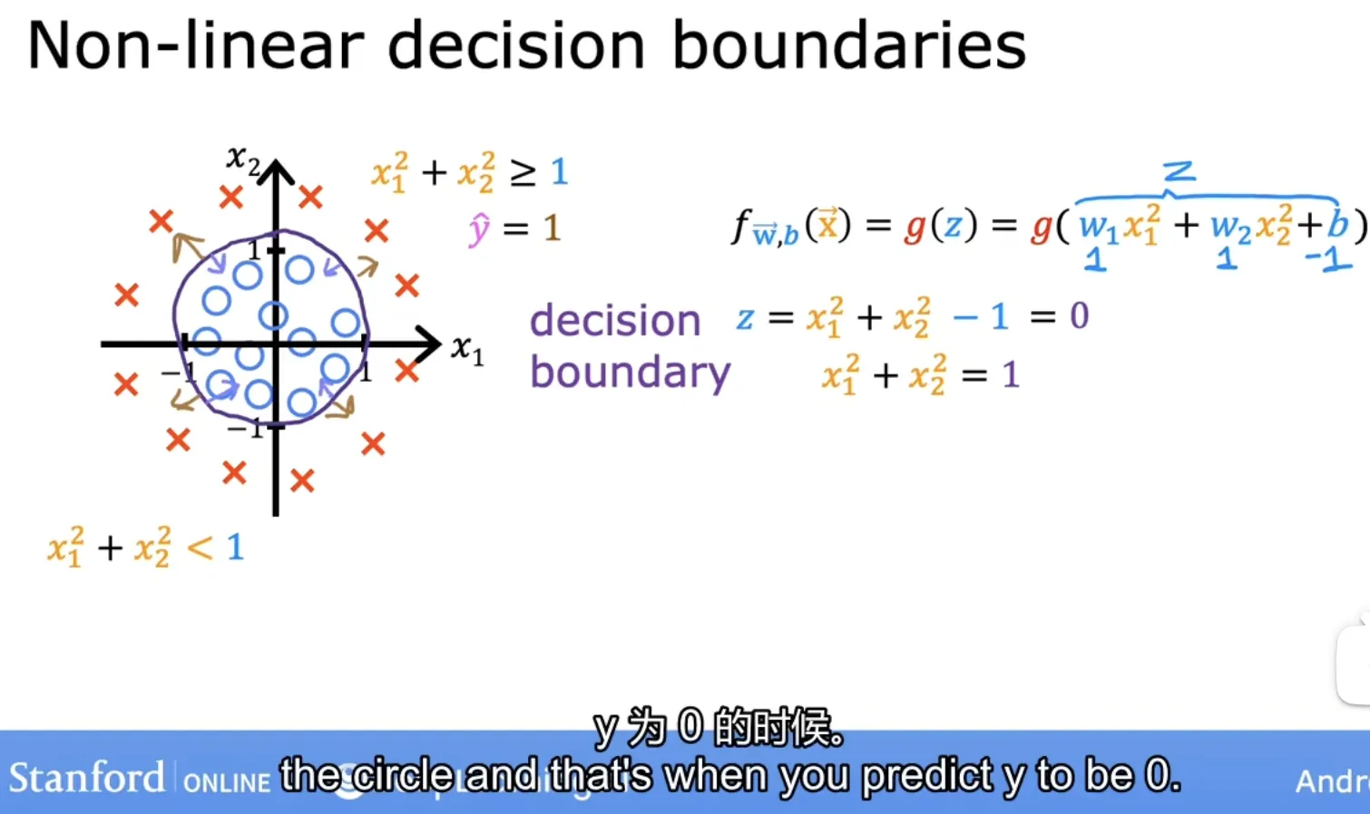
多項式邏輯回歸
多項式回歸決策邊界,我們假設:
- 多項式模型:
z = w1 * x1**2 + w2 * x2**2 + b - 參數:
w1=w2=1, b=-1
如果特征x在圓的外面,那么此邏輯回歸則預測為1,反之則預測為0;(分為兩類)
擴展:隨著多項式的復雜度增加,還可以擬合更更多非線性的復雜情況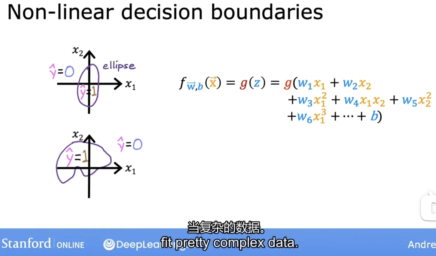
邏輯回歸的損失函數
平方損失和交叉熵損失
回顧下線性回歸的損失函數(平方損失):
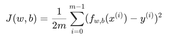
平方誤差損失函數不適用于邏輯回歸模型:平方損失在邏輯回歸中是 “非凸函數”(存在多個局部最優解),難以優化;
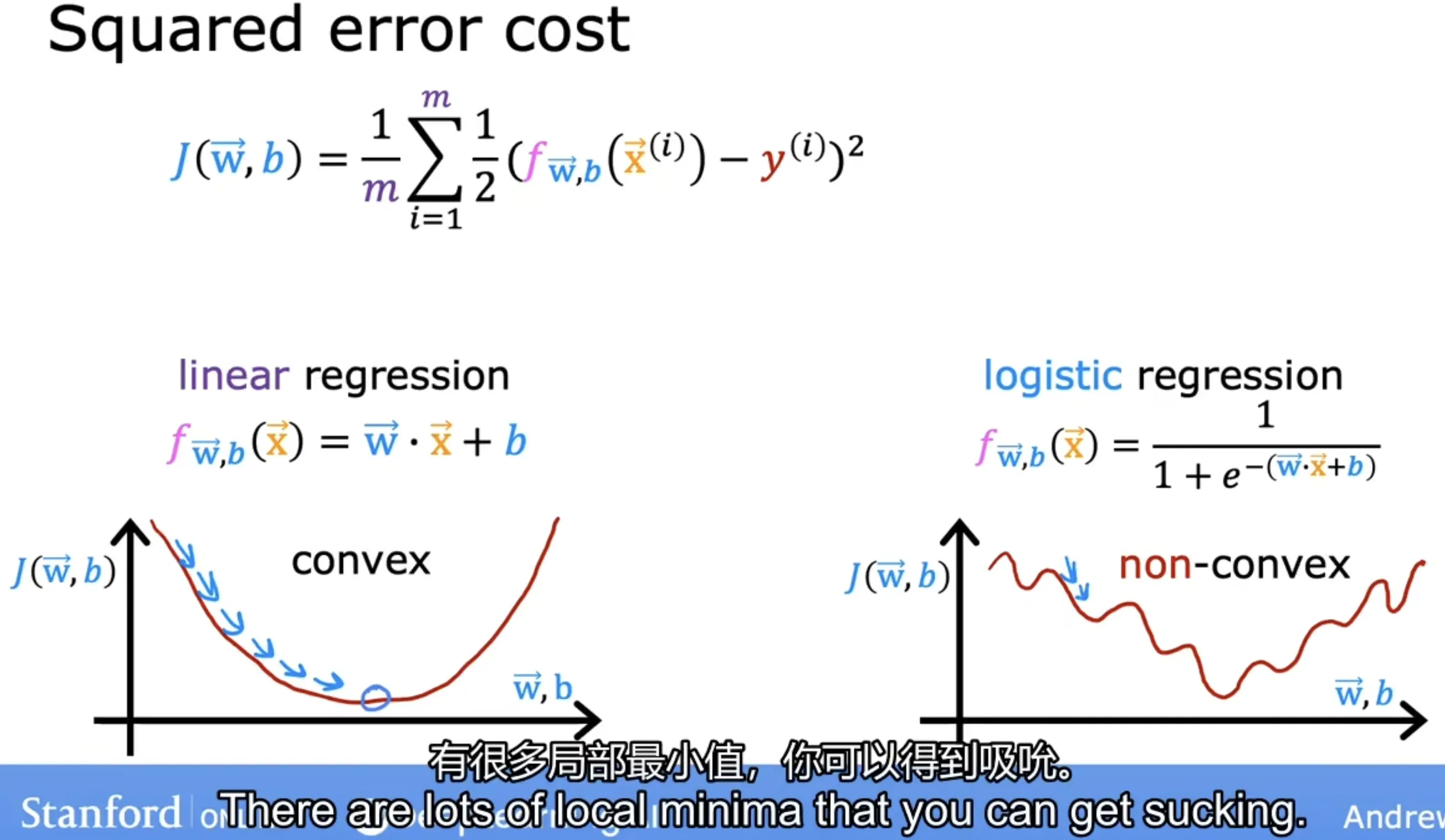
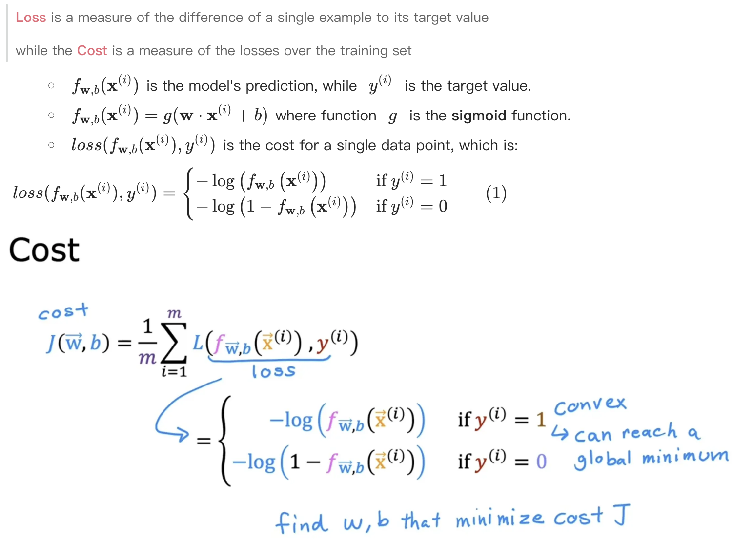
所以我們需要一個新的損失函數,即交叉熵損失;交叉熵損失是 “凸函數”,可通過梯度下降高效找到全局最優。
交叉熵源于信息論,我們暫時不做深入介紹,直接給出交叉熵損失函數公式:
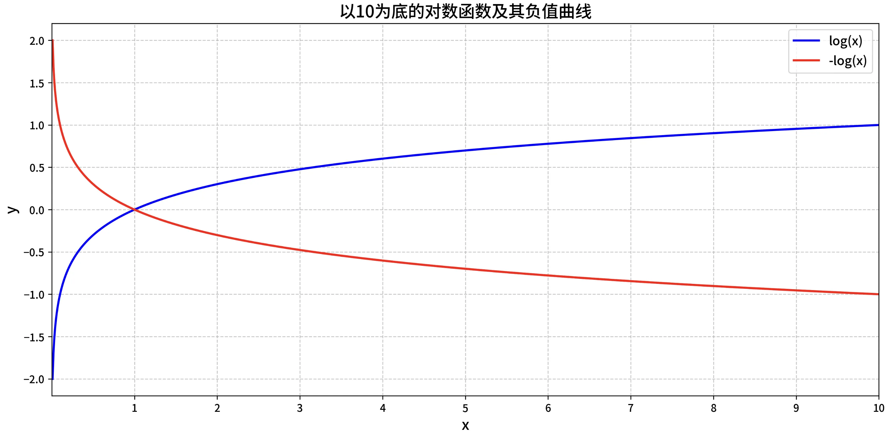
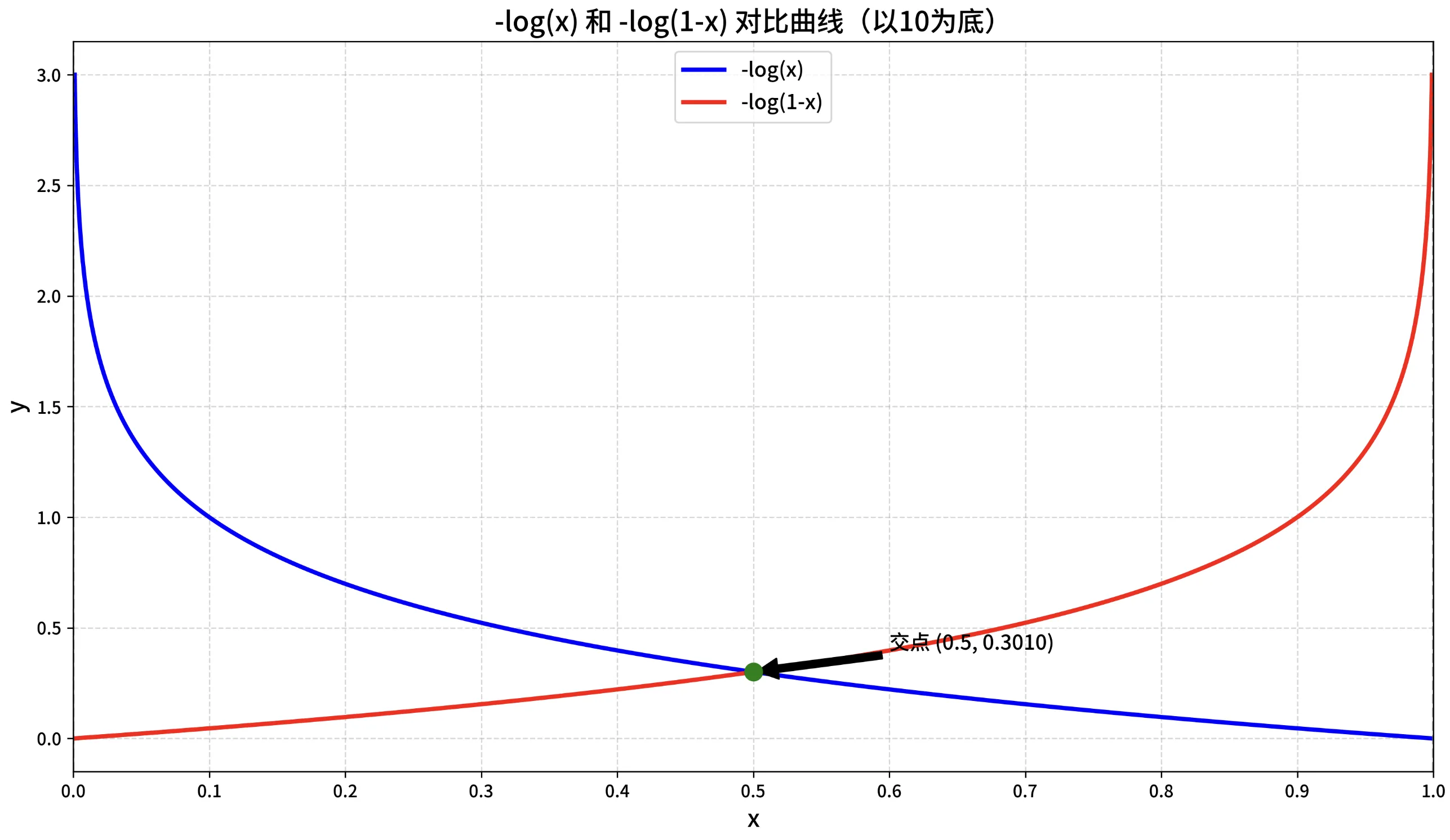
對數回顧
復習下對數函數的性質,以便理解為什么 交叉熵損失是 “凸函數”?
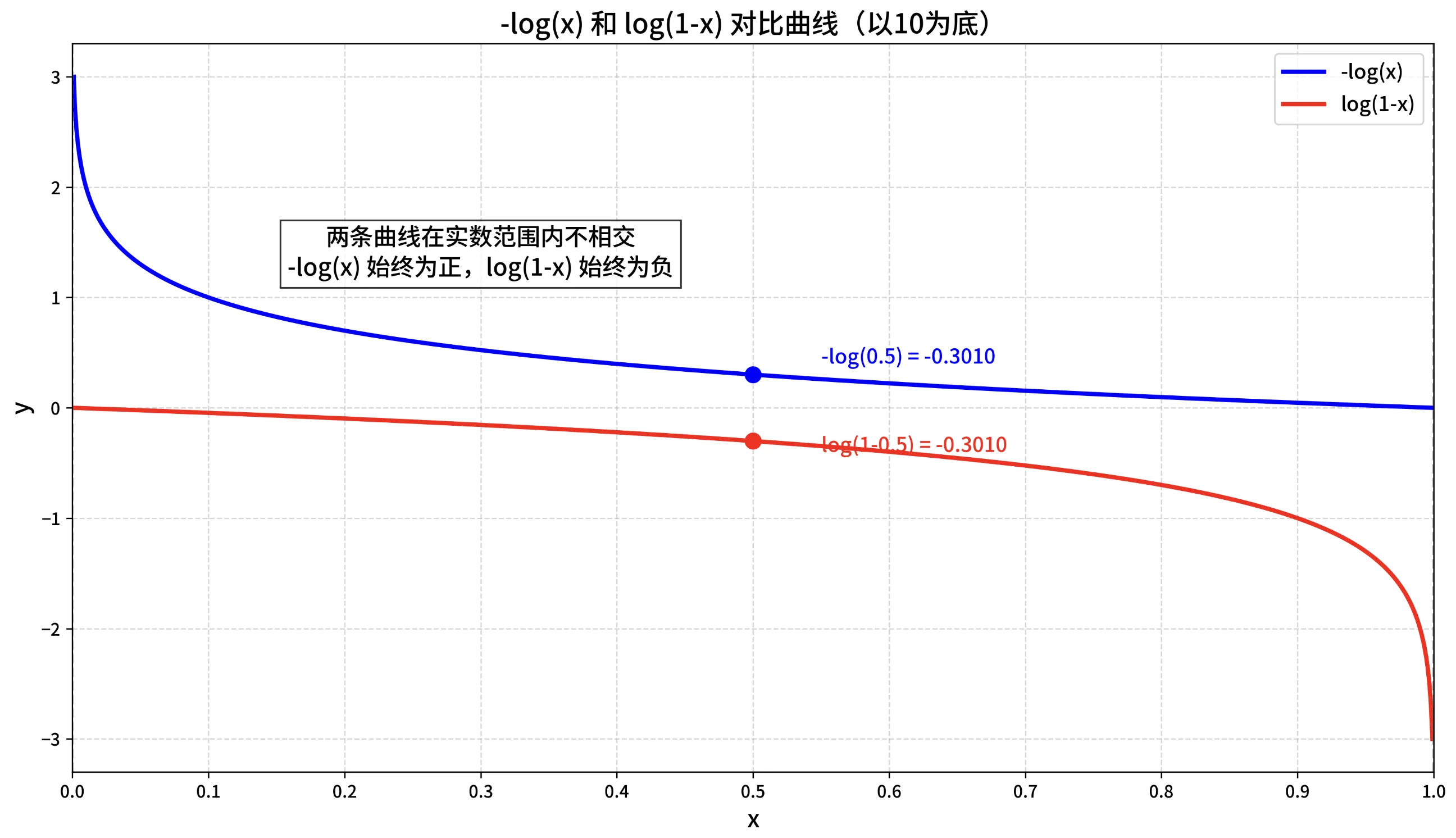
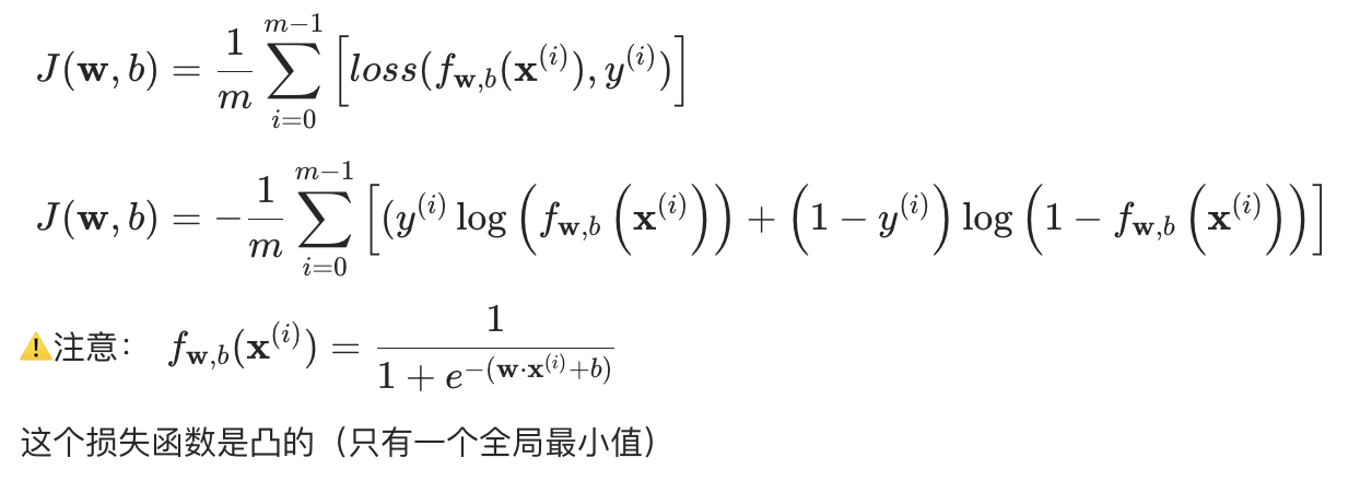
簡化交叉熵損失函數
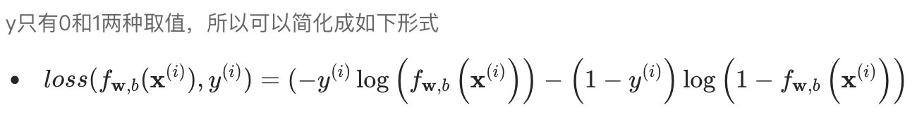
為什么要用這個函數來表示?來源自 最大釋然估計(Maximum Likelihood),這里不做過多介紹。
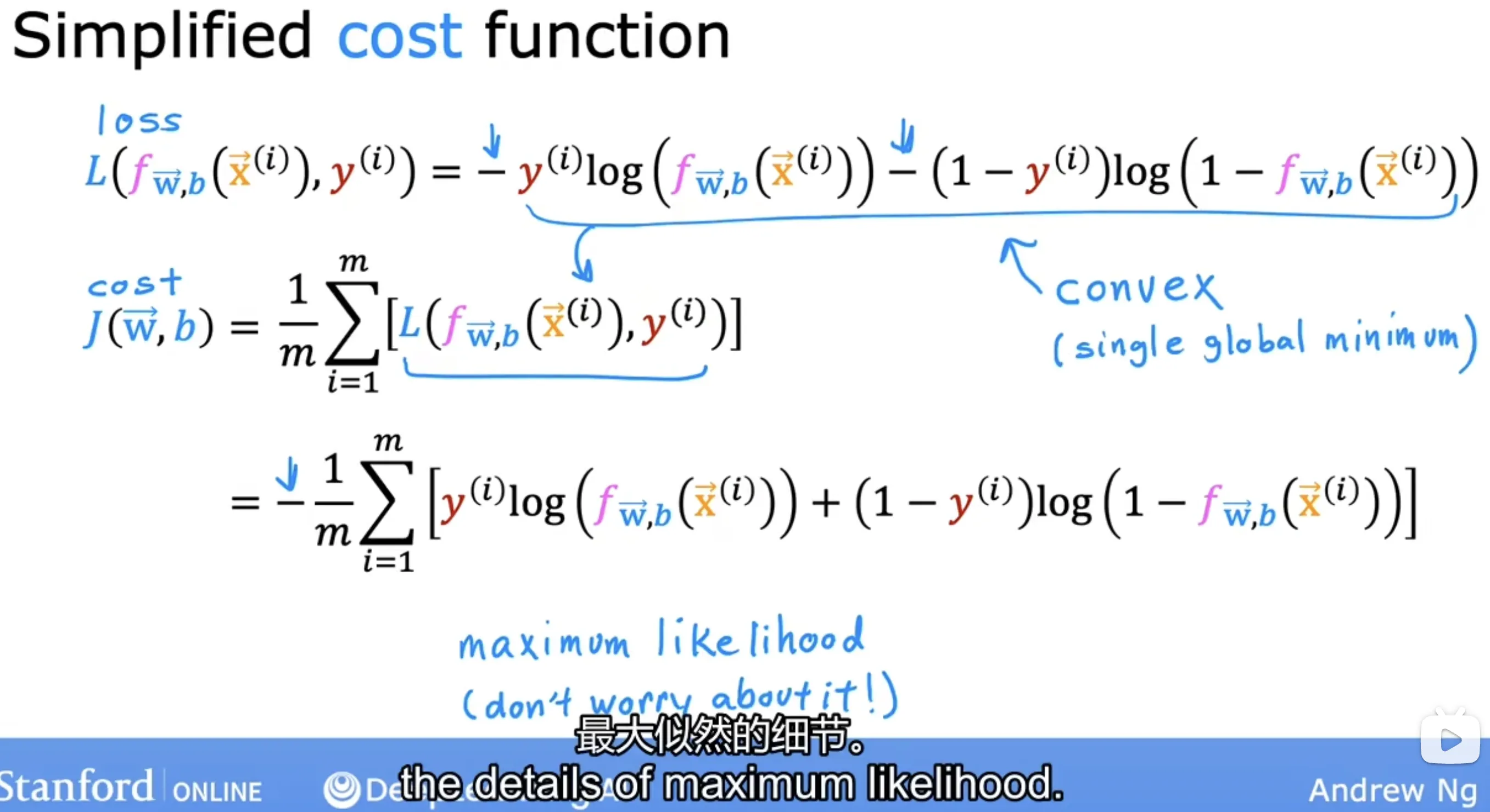
簡化結果:
邏輯回歸的梯度計算
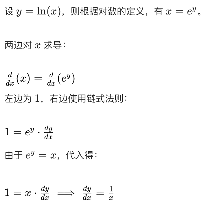
自然對數求導公式:
鏈式求導法則:
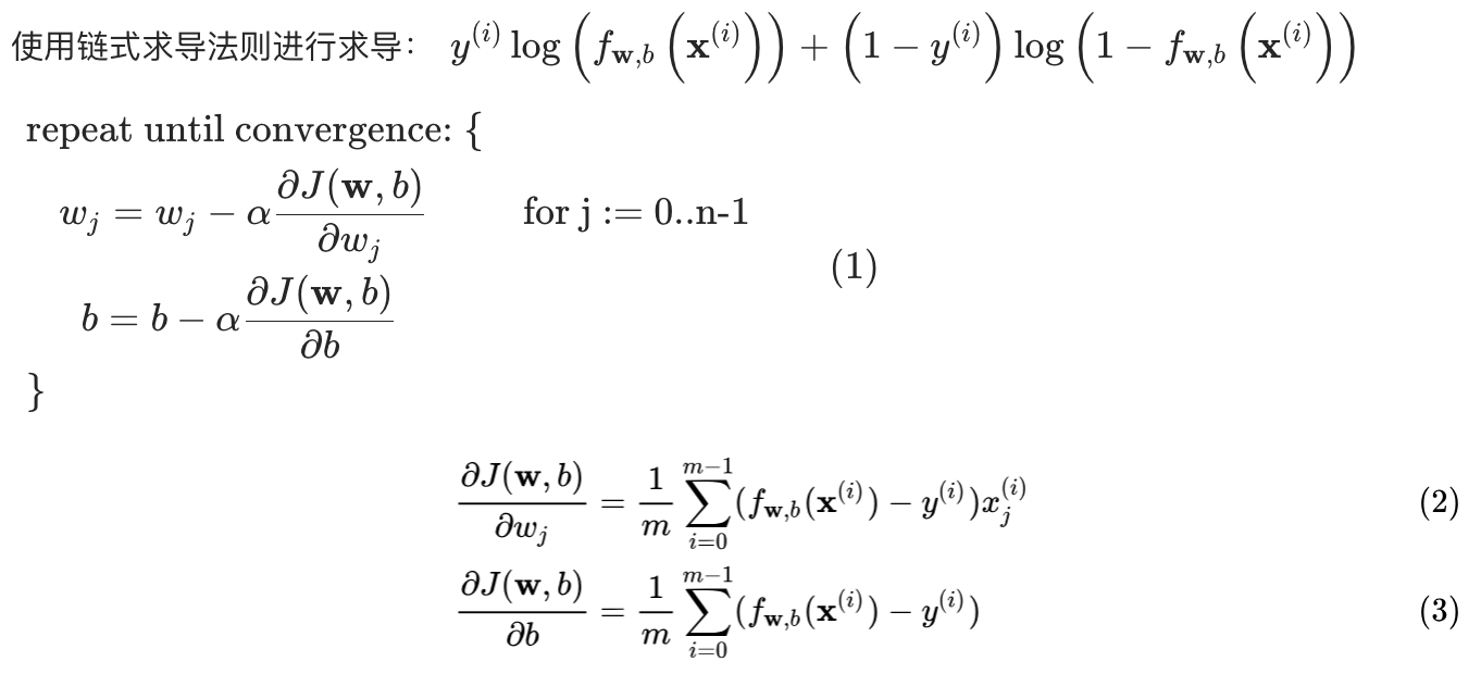
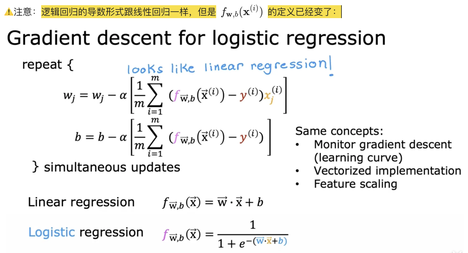
??注意:
過擬合問題
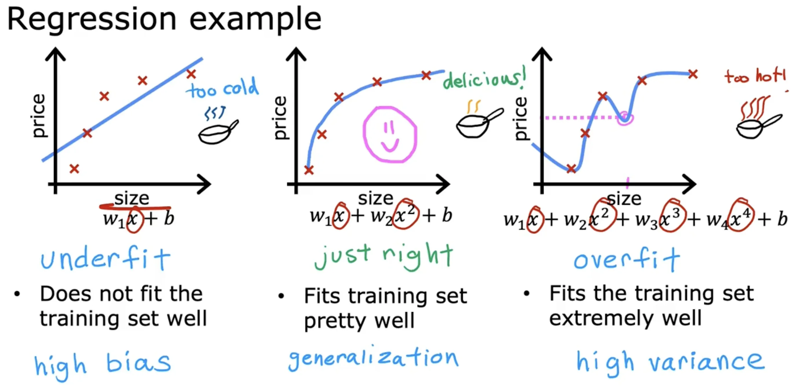
線性回歸過擬合
邏輯回歸過擬合
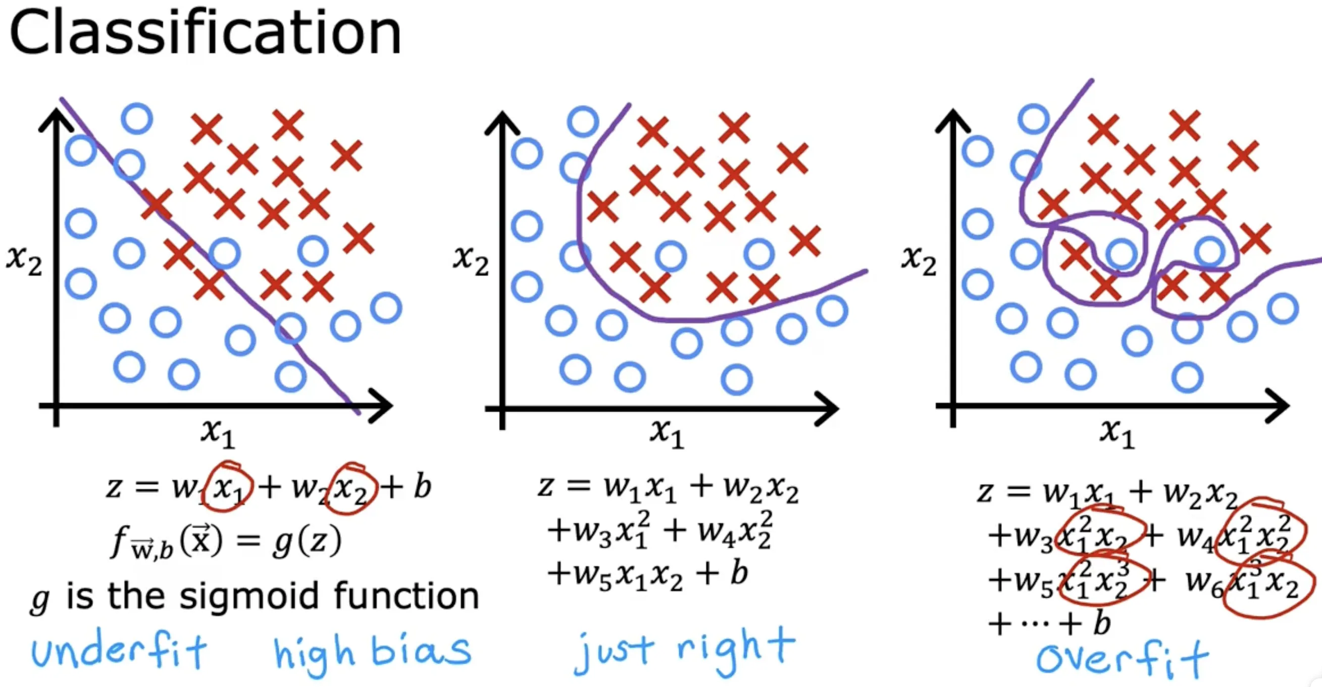
- 欠擬合(underfit),存在高偏差(bias)
- 泛化(generalization):希望我們的學習算法在訓練集之外的數據上也能表現良好(預測準確)
- 過擬合(overfit),存在高方差(variance)
解決過擬合的辦法
- 特征選擇:只選擇部分最相關的特征(基于直覺intuition)進行訓練;缺點是丟掉了部分可能有用的信息
- 正則化:正則化是一種更溫和的減少某些特征的影響,而無需做像測地消除它那樣苛刻的事:
- 鼓勵學習算法縮小參數,而不是直接將參數設置為0(保留所有特征的同時避免讓部分特征產生過大的影響)
- 鼓勵把 w1 ~ wn 變小,b不用變小
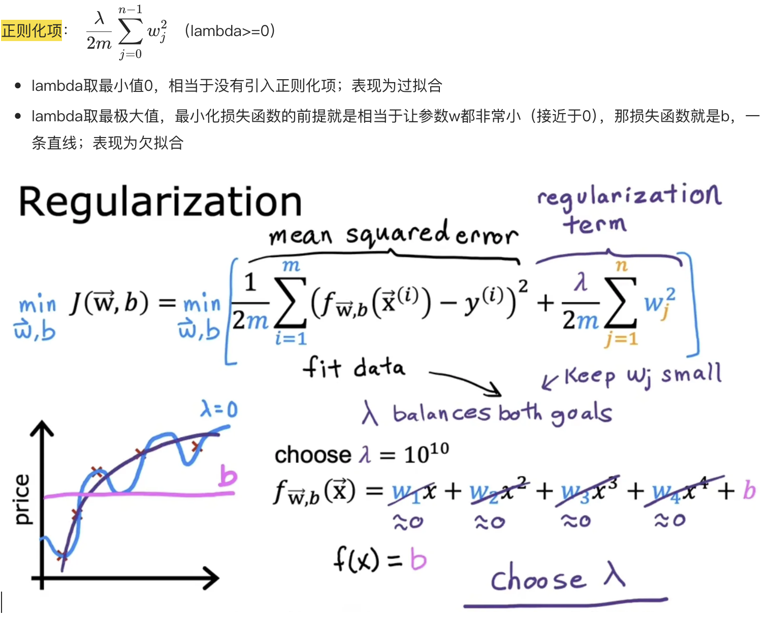
正則化模型
It turns out that regularization is a way
to more gently reduce ths impacts of some of the features without doing something as harsh as eliminating it outright.

關于正則化項的說明:
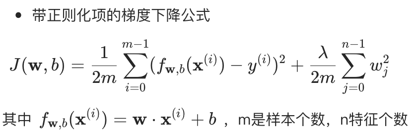
帶正則化項的損失函數
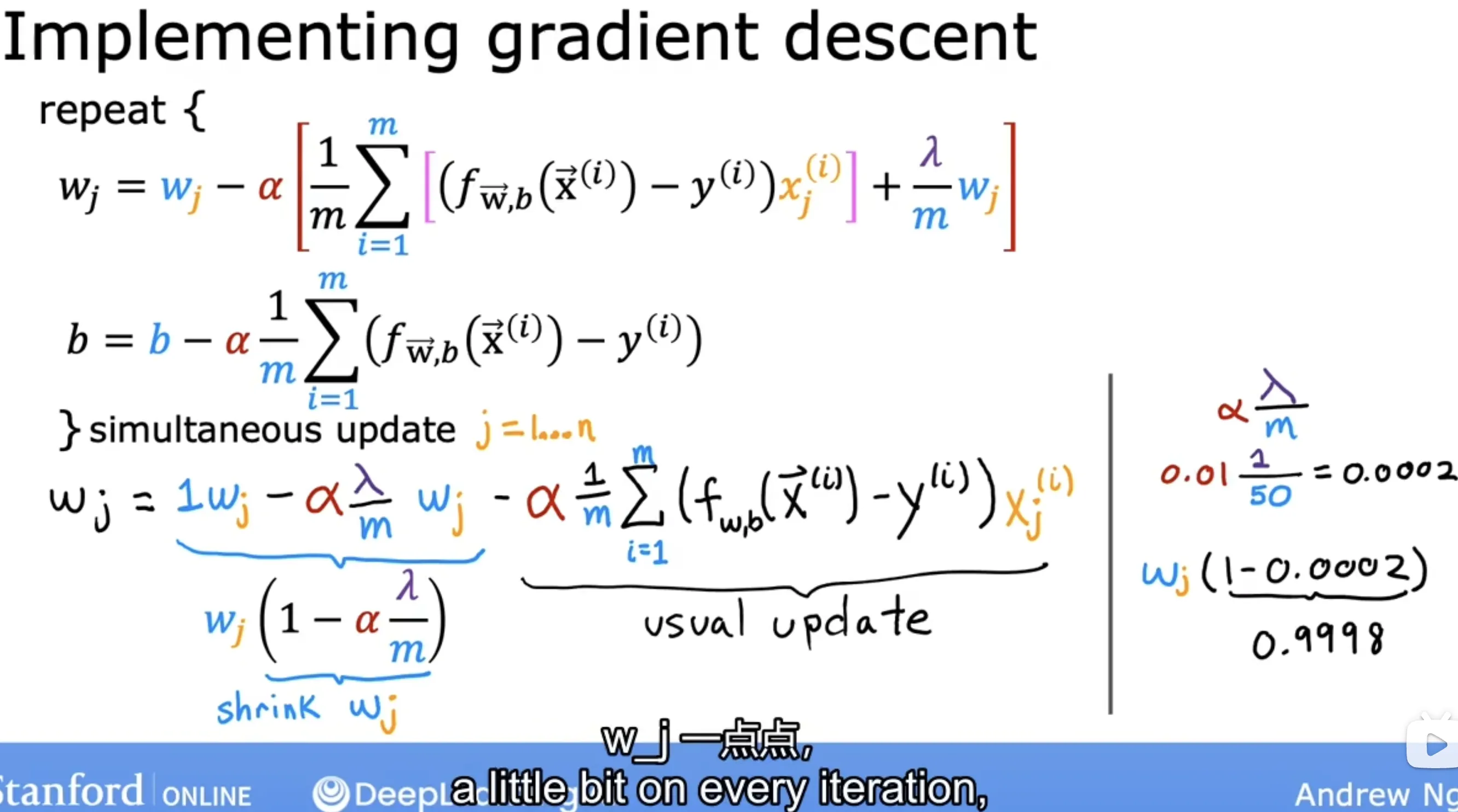
正則化線性回歸
損失函數:
梯度計算:
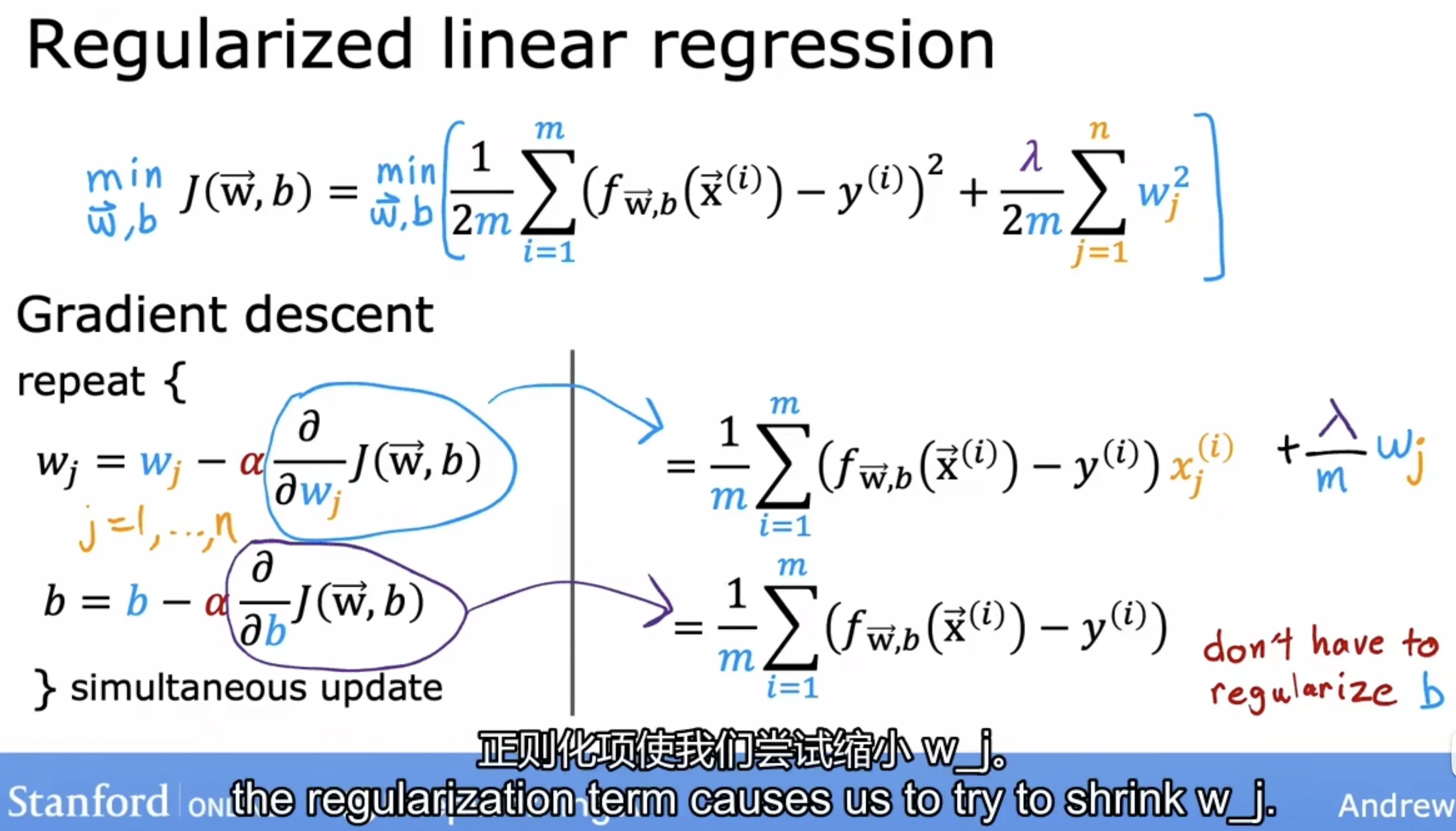
分析梯度計算公式,由于alpha和lambda通常是很小的值,所以相當于在每次迭代之前把參數w縮小了一點點,這也就是正則化的工作原理,如下所示:
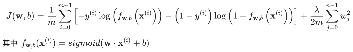
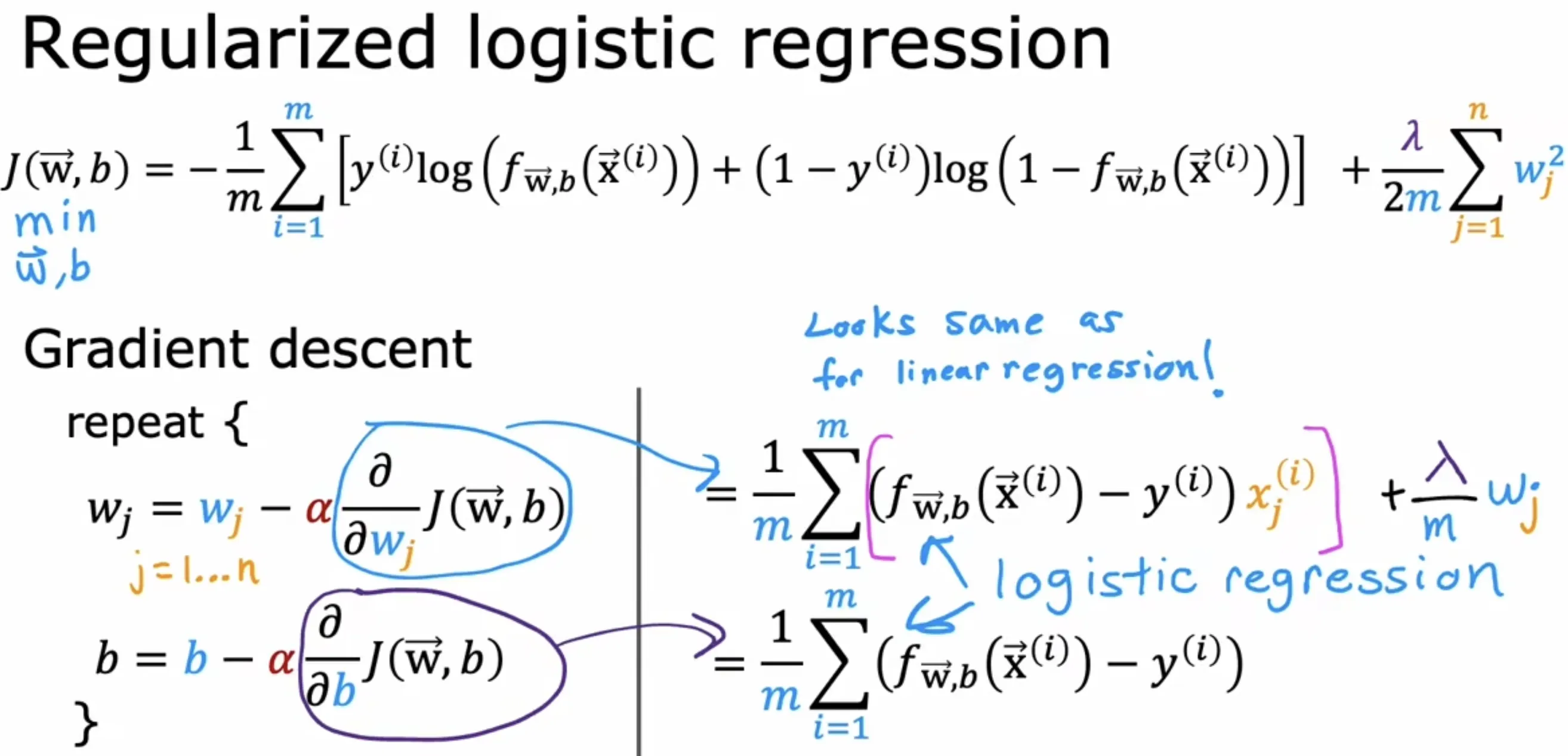
正則化邏輯回歸
損失函數:
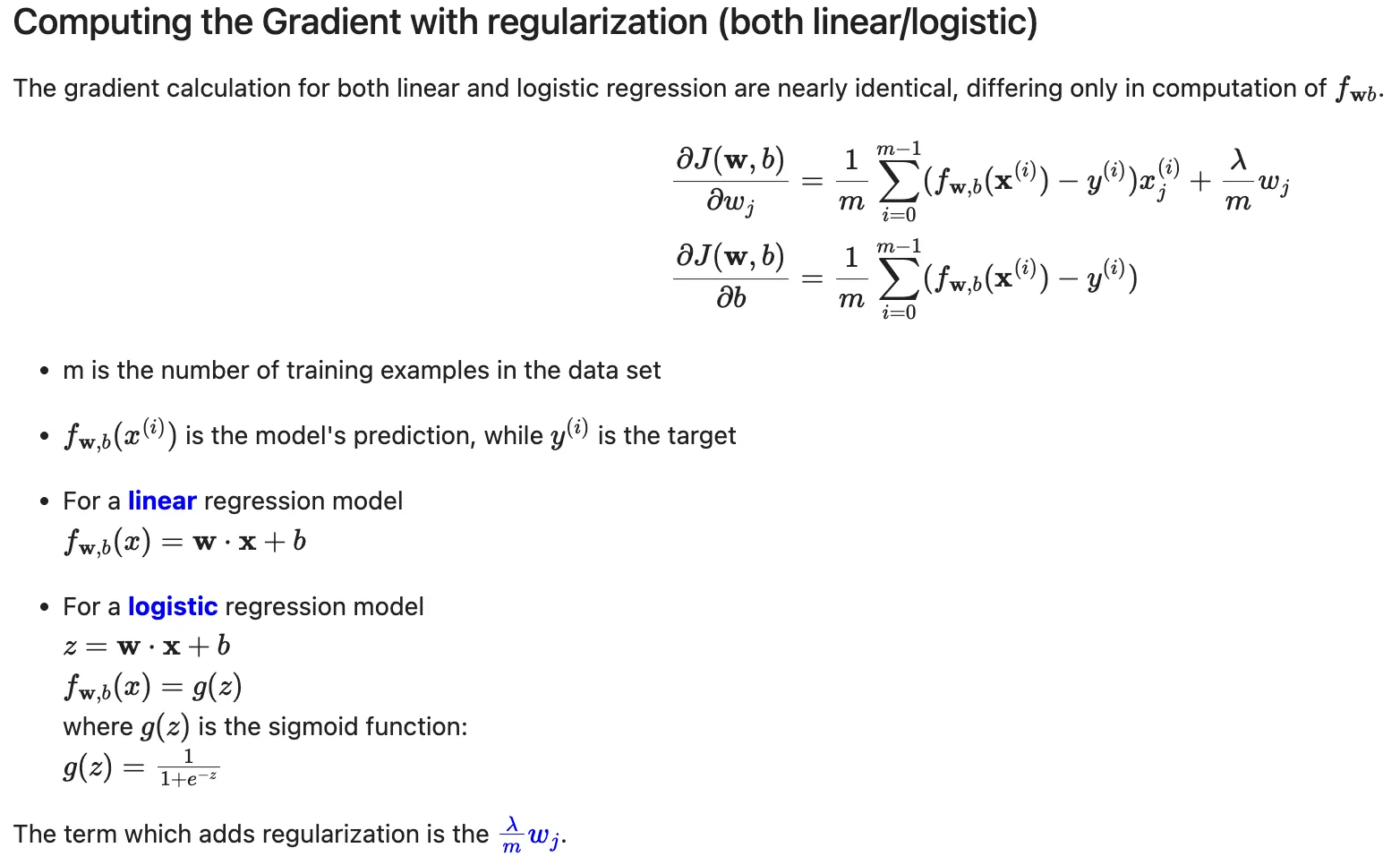
梯度計算:
線性回歸和邏輯回歸正則化總結
邏輯回歸實戰
模型選擇
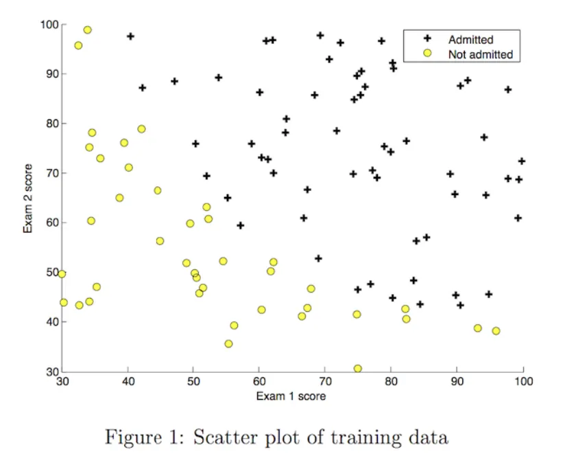
可視化訓練數據,基于此數據選擇線性邏輯回歸模型
關鍵代碼實現
def sigmoid(z):
	g = 1 / (1 + np.exp(-z))
	return g

def compute_cost(X, y, w, b, lambda_= 1):
	"""
    Computes the cost over all examples
    Args:
      X : (ndarray Shape (m,n)) data, m examples by n features
      y : (array_like Shape (m,)) target value
      w : (array_like Shape (n,)) Values of parameters of the model
      b : scalar Values of bias parameter of the model
      lambda_: unused placeholder
    Returns:
      total_cost: (scalar)         cost
    """

	m, n = X.shape
	total_cost = 0
	for i in range(m):
		f_wb_i = sigmoid(np.dot(X[i], w) + b)
		loss = -y[i] * np.log(f_wb_i) - (1 - y[i]) * np.log(1 - f_wb_i)
		total_cost += loss

	total_cost = total_cost / m
	return total_cost

def compute_gradient(X, y, w, b, lambda_=None):
    """
    Computes the gradient for logistic regression

    Args:
      X : (ndarray Shape (m,n)) variable such as house size
      y : (array_like Shape (m,1)) actual value
      w : (array_like Shape (n,1)) values of parameters of the model
      b : (scalar)                 value of parameter of the model
      lambda_: unused placeholder.
    Returns
      dj_dw: (array_like Shape (n,1)) The gradient of the cost w.r.t. the parameters w.
      dj_db: (scalar)                The gradient of the cost w.r.t. the parameter b.
    """
    m, n = X.shape
    dj_dw = np.zeros(n)
    dj_db = 0.

    for i in range(m):
        f_wb_i = sigmoid(np.dot(X[i], w) + b)
        diff = f_wb_i - y[i]
        dj_db += diff
        for j in range(n):
            dj_dw[j] = dj_dw[j] + diff * X[i][j]

    dj_db = dj_db / m
    dj_dw = dj_dw / m

    return dj_db, dj_dw

def gradient_descent(X, y, w_in, b_in, cost_function, gradient_function, alpha, num_iters, lambda_):
    """
    Performs batch gradient descent to learn theta. Updates theta by taking
    num_iters gradient steps with learning rate alpha

    Args:
      X :    (array_like Shape (m, n)
      y :    (array_like Shape (m,))
      w_in : (array_like Shape (n,))  Initial values of parameters of the model
      b_in : (scalar)                 Initial value of parameter of the model
      cost_function:                  function to compute cost
      alpha : (float)                 Learning rate
      num_iters : (int)               number of iterations to run gradient descent
      lambda_ (scalar, float)         regularization constant

    Returns:
      w : (array_like Shape (n,)) Updated values of parameters of the model after
          running gradient descent
      b : (scalar)                Updated value of parameter of the model after
          running gradient descent
    """

    # number of training examples
    m = len(X)

    # An array to store cost J and w's at each iteration primarily for graphing later
    J_history = []
    w_history = []

    w = copy.deepcopy(w_in)
    b = b_in

    for i in range(num_iters):
        dj_db, dj_dw = gradient_function(X, y, w, b, lambda_)
        w = w - alpha * dj_dw
        b = b - alpha * dj_db
        cost = cost_function(X, y, w, b, lambda_)
        J_history.append(cost)
        w_history.append(w)
        if i % math.ceil(num_iters / 10) == 0:
            print(f"{i:4d} cost: {cost:6f}, w: {w}, b: {b}")

    return w, b, J_history, w_history #return w and J,w history for graphing


def predict(X, w, b):
    m, n = X.shape
    p = np.zeros(m)
    for i in range(m):
        f_wb = sigmoid(np.dot(X[i], w) + b)
        p[i] = f_wb >= 0.5
    return p
結果展示
import numpy as np
import matplotlib.pyplot as plt
import matplotlib.font_manager as fm
# 支持顯示中文
font_path = '/System/Library/Fonts/STHeiti Light.ttc'
custom_font = fm.FontProperties(fname=font_path)
plt.rcParams["font.family"] = custom_font.get_name()
# 載入訓練集
X_train, y_train = load_data("data/ex2data1.txt")
# 訓練模型
np.random.seed(1)
intial_w = 0.01 * (np.random.rand(2).reshape(-1,1) - 0.5)
initial_b = -8
iterations = 10000
alpha = 0.001
w_out, b_out, J_history,_ = gradient_descent(X_train ,y_train, initial_w, initial_b, compute_cost, compute_gradient, alpha, iterations, 0)
# 根據訓練結果(w_out和b_out)計算決策邊界
#f = w0*x0 + w1*x1 + b
# x1 = -1 * (w0*x0 + b) / w1
plot_x = np.array([min(X_train[:, 0]), max(X_train[:, 0])])
plot_y = (-1. / w_out[1]) * (w_out[0] * plot_x + b_out)
# 將訓練數據分類
x0s_pos = []
x1s_pos = []
x0s_neg = []
x1s_neg = []
for i in range(len(X_train)):
x = X_train[i]
# print(x)
y_i = y_train[i]
if y_i == 1:
x0s_pos.append(x[0])
x1s_pos.append(x[1])
else:
x0s_neg.append(x[0])
x1s_neg.append(x[1])
# 繪圖
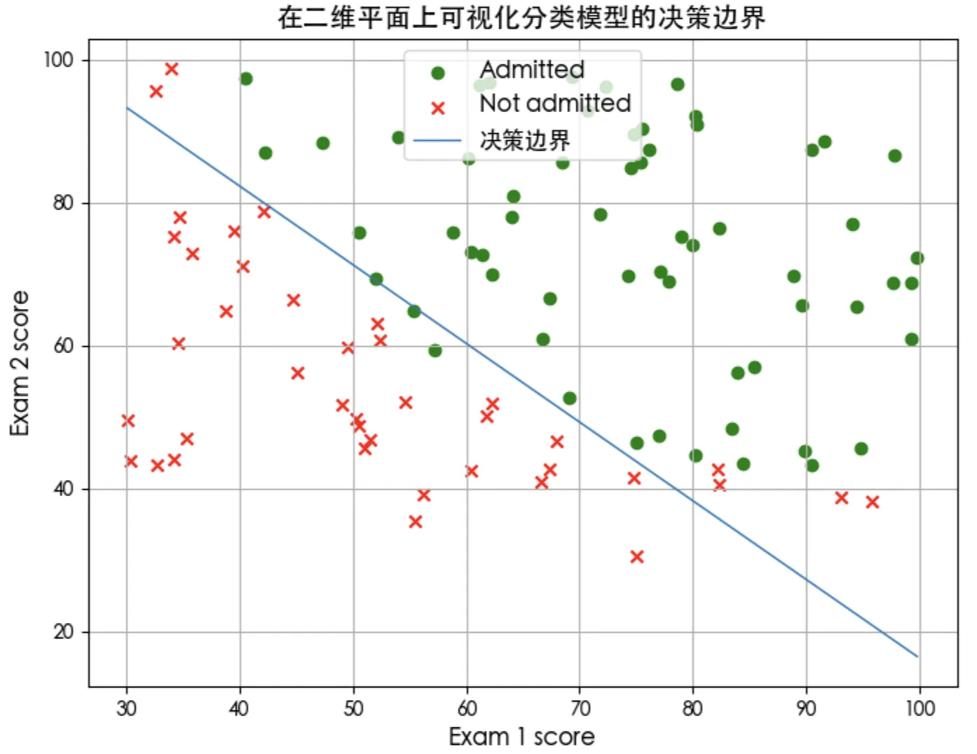
plt.figure(figsize=(8, 6))
plt.scatter(x0s_pos, x1s_pos, marker='o', c='green', label="Admitted")
plt.scatter(x0s_neg, x1s_neg, marker='x', c='red', label="Not admitted")
plt.plot(plot_x, plot_y, lw=1, label="決策邊界")
plt.xlabel('Exam 1 score', fontsize=12)
plt.ylabel('Exam 2 score', fontsize=12)
plt.title('在二維平面上可視化分類模型的決策邊界', fontsize=14)
plt.legend(fontsize=12, loc='upper center')
plt.grid(True)
plt.show()
# 使用訓練集計算預測準確率
p = predict(X_train, w_out, b_out)
print('Train Accuracy: %f'%(np.mean(p == y_train) * 100))
# Train Accuracy: 92.000000
正則化邏輯回歸實戰
模型選擇
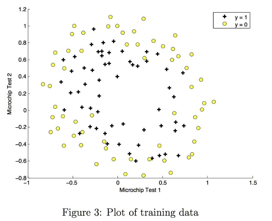
可視化訓練數據,基于此數據選擇多項式邏輯回歸模型
關鍵代碼實現
由于要擬合非線性決策邊界,所以要增加特征的復雜度(訓練數據里只有2個特征)。
特征映射函數
# 將輸入特征 X1 和 X2 轉換為六次多項式特征
# 這個函數常用于邏輯回歸或支持向量機等模型中,通過增加特征的復雜度來擬合非線性決策邊界。
def map_feature(X1, X2):
    """
    Feature mapping function to polynomial features
    """
    X1 = np.atleast_1d(X1)
    X2 = np.atleast_1d(X2)
    degree = 6
    out = []
    for i in range(1, degree+1):
        for j in range(i + 1):
            out.append((X1**(i-j) * (X2**j)))
    return np.stack(out, axis=1)
正則化后的損失函數和梯度計算函數
def compute_cost_reg(X, y, w, b, lambda_ = 1):
    """
    Computes the cost over all examples
    Args:
      X : (array_like Shape (m,n)) data, m examples by n features
      y : (array_like Shape (m,)) target value
      w : (array_like Shape (n,)) Values of parameters of the model
      b : (array_like Shape (n,)) Values of bias parameter of the model
      lambda_ : (scalar, float)    Controls amount of regularization
    Returns:
      total_cost: (scalar)         cost
    """
    m, n = X.shape
    # Calls the compute_cost function that you implemented above
    cost_without_reg = compute_cost(X, y, w, b)

    reg_cost = 0.
    for j in range(n):
        reg_cost += w[j]**2

    # Add the regularization cost to get the total cost
    total_cost = cost_without_reg + (lambda_/(2 * m)) * reg_cost

    return total_cost

def compute_gradient_reg(X, y, w, b, lambda_ = 1):
    """
    Computes the gradient for linear regression

    Args:
      X : (ndarray Shape (m,n))   variable such as house size
      y : (ndarray Shape (m,))    actual value
      w : (ndarray Shape (n,))    values of parameters of the model
      b : (scalar)                value of parameter of the model
      lambda_ : (scalar,float)    regularization constant
    Returns
      dj_db: (scalar)             The gradient of the cost w.r.t. the parameter b.
      dj_dw: (ndarray Shape (n,)) The gradient of the cost w.r.t. the parameters w.

    """
    m, n = X.shape

    dj_db, dj_dw = compute_gradient(X, y, w, b)

    # Add the regularization
    for j in range(n):
        dj_dw[j] += (lambda_ / m) * w[j]

    return dj_db, dj_dw
結果展示
import numpy as np
import matplotlib.pyplot as plt
import matplotlib.font_manager as fm
# 支持顯示中文
font_path = '/System/Library/Fonts/STHeiti Light.ttc'
custom_font = fm.FontProperties(fname=font_path)
plt.rcParams["font.family"] = custom_font.get_name()
# 載入訓練集
X_train, y_train = load_data("data/ex2data2.txt")
# 通過增加特征的復雜度來擬合非線性決策邊界
X_mapped = map_feature(X_train[:, 0], X_train[:, 1])
print("Original shape of data:", X_train.shape)
print("Shape after feature mapping:", X_mapped.shape)
# 訓練模型
np.random.seed(1)
initial_w = np.random.rand(X_mapped.shape[1])-0.5
initial_b = 1.
# Set regularization parameter lambda_ to 1 (you can try varying this)
lambda_ = 0.5
iterations = 10000
alpha = 0.01
w_out, b_out, J_history, _ = gradient_descent(X_mapped, y_train, initial_w, initial_b, compute_cost_reg, compute_gradient_reg, alpha, iterations, lambda_)
# 根據訓練結果(w_out和b_out)計算決策邊界
# - 創建網格點 u 和 v 覆蓋特征空間
u = np.linspace(-1, 1.5, 50)
v = np.linspace(-1, 1.5, 50)
# - 計算每個網格點處的預測概率 z
z = np.zeros((len(u), len(v)))
# Evaluate z = theta*x over the grid
for i in range(len(u)):
for j in range(len(v)):
z[i,j] = sig(np.dot(map_feature(u[i], v[j]), w_out) + b_out)
# - 轉置 z 是必要的,因為contour函數期望的輸入格式與我們的計算順序不一致
z = z.T
# 分類
x0s_pos = []
x1s_pos = []
x0s_neg = []
x1s_neg = []
for i in range(len(X_train)):
x = X_train[i]
# print(x)
y_i = y_train[i]
if y_i == 1:
x0s_pos.append(x[0])
x1s_pos.append(x[1])
else:
x0s_neg.append(x[0])
x1s_neg.append(x[1])
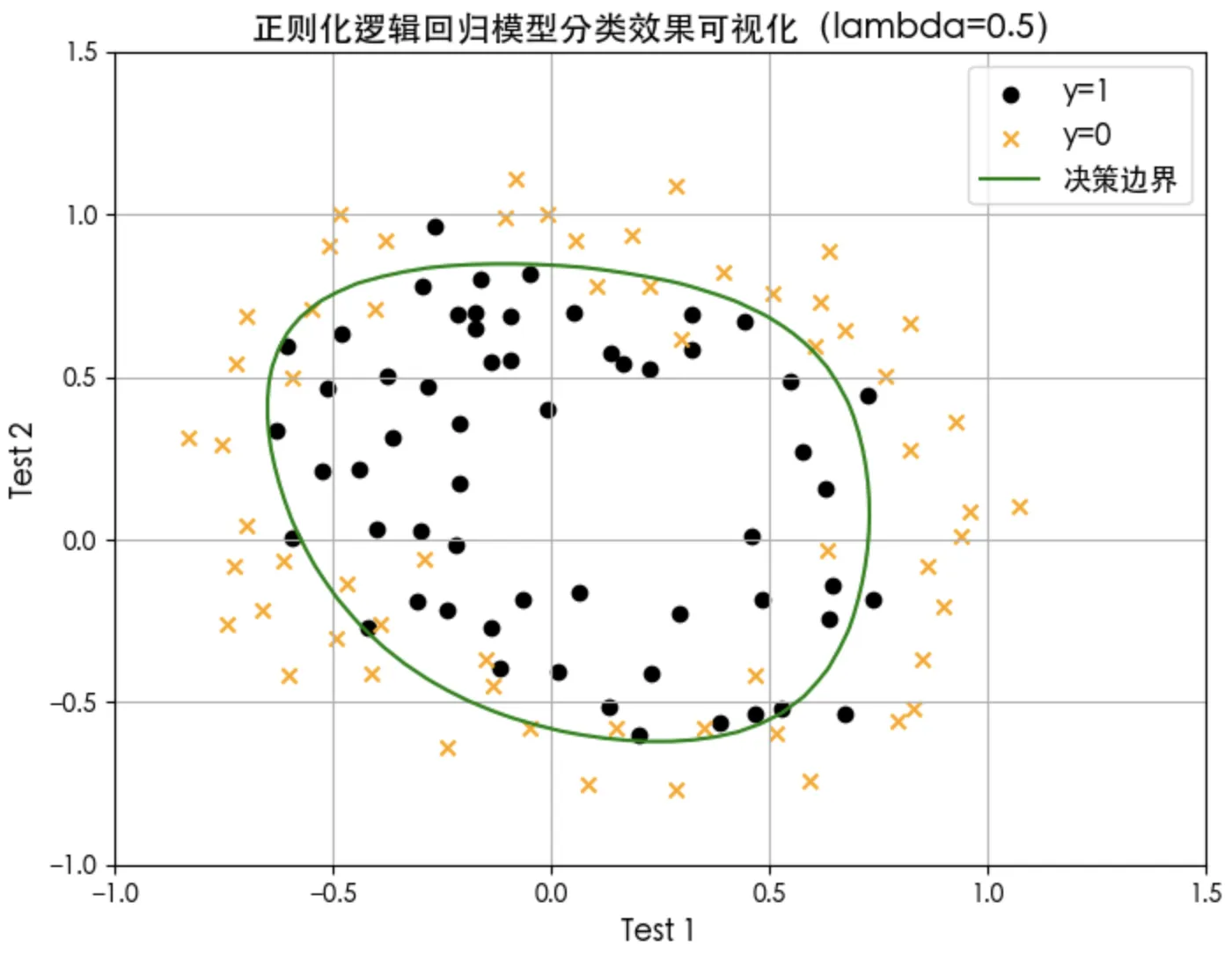
# 繪圖
plt.figure(figsize=(8, 6))
plt.scatter(x0s_pos, x1s_pos, marker='o', c='black', label="y=1")
plt.scatter(x0s_neg, x1s_neg, marker='x', c='orange', label="y=0")
# 繪制決策邊界(等高線)
plt.contour(u,v,z, levels = [0.5], colors="green")
# 創建虛擬線條用于圖例(顏色和線型需與等高線一致)
plt.plot([], [], color='green', label="決策邊界")
plt.xlabel('Test 1', fontsize=12)
plt.ylabel('Test 2', fontsize=12)
plt.title('正則化邏輯回歸模型分類效果可視化(lambda=0.5)', fontsize=14)
# plt.legend(fontsize=12, loc='upper center')
plt.legend(fontsize=12)
plt.grid(True)
plt.show()
#Compute accuracy on the training set
p = predict(X_mapped, w_out, b_out)
print('Train Accuracy: %f'%(np.mean(p == y_train) * 100))
# Train Accuracy: 83.050847
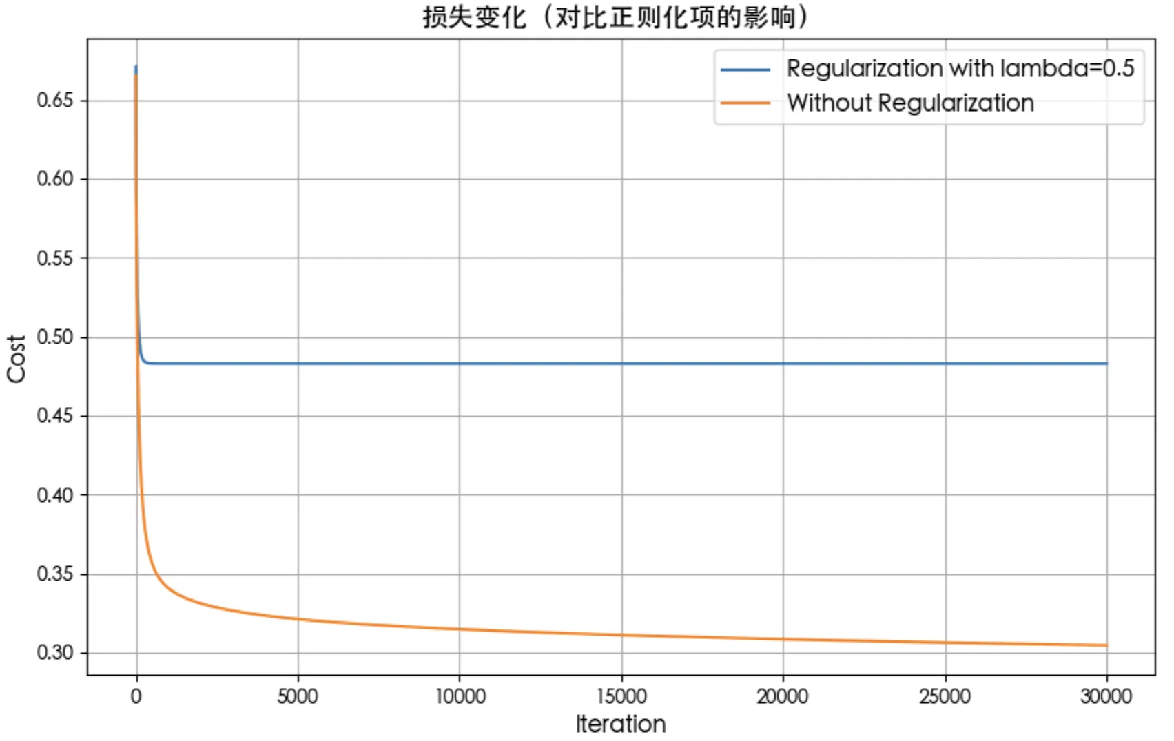
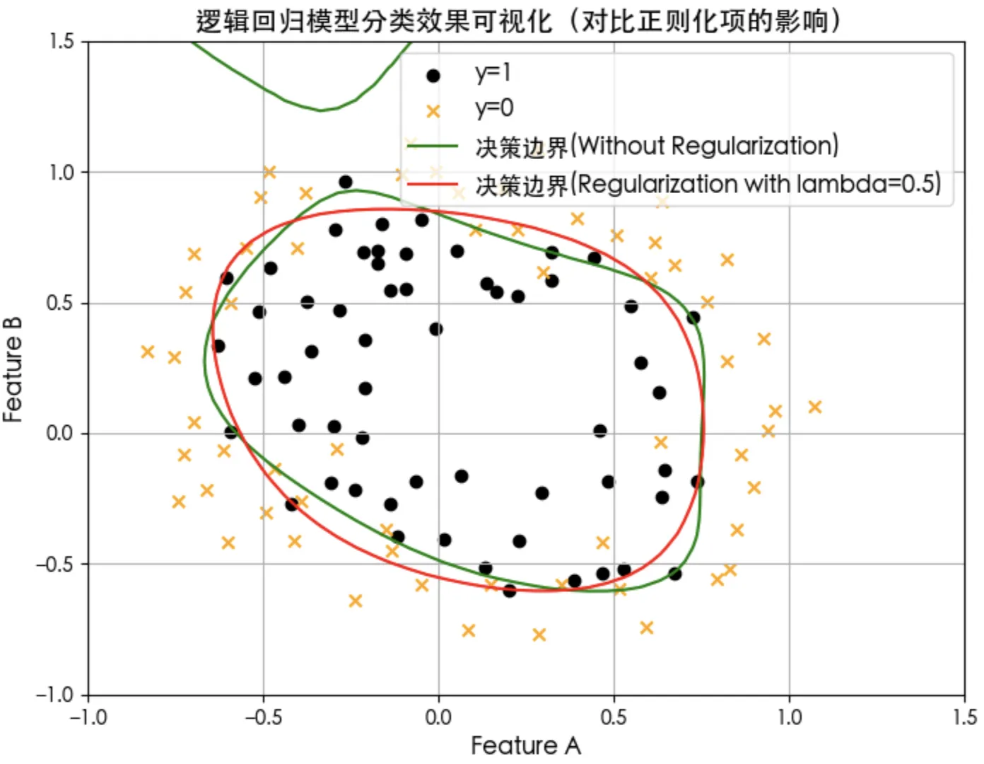
正則化效果對比
正則化對損失和決策邊界的影響
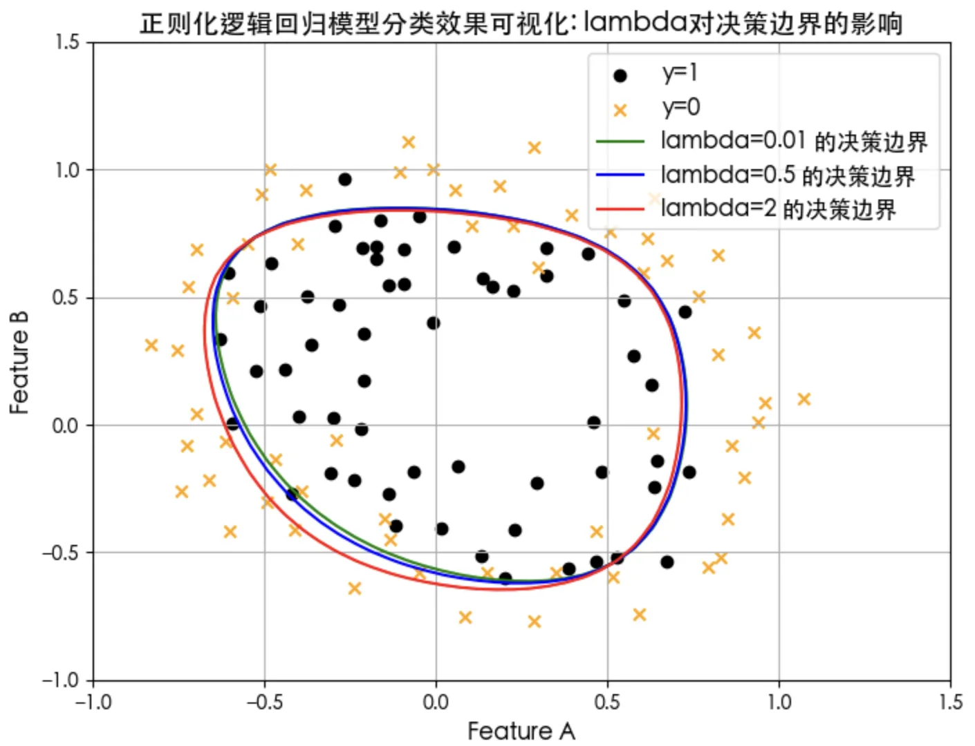
正則化項lambda參數大小對決策邊界的影響
參考
吳恩達團隊在Coursera開設的機器學習課程:https://www.coursera.org/specializations/machine-learning-introduction
在B站學習:https://www.bilibili.com/video/BV1Pa411X76s
出處:http://www.rzrgm.cn/standby/
本文版權歸作者和博客園共有,歡迎轉載,但未經作者同意必須保留此段聲明,且在文章頁面明顯位置給出原文連接,否則保留追究法律責任的權利。

 浙公網安備 33010602011771號