量化曲線的平滑程度
思路
1. 對原始數據一階求導,得到一階導數數組。
2. 對一階導數數組求標準差。導數的標準差提供了導數值的波動性,標準差越小,曲線越平滑。
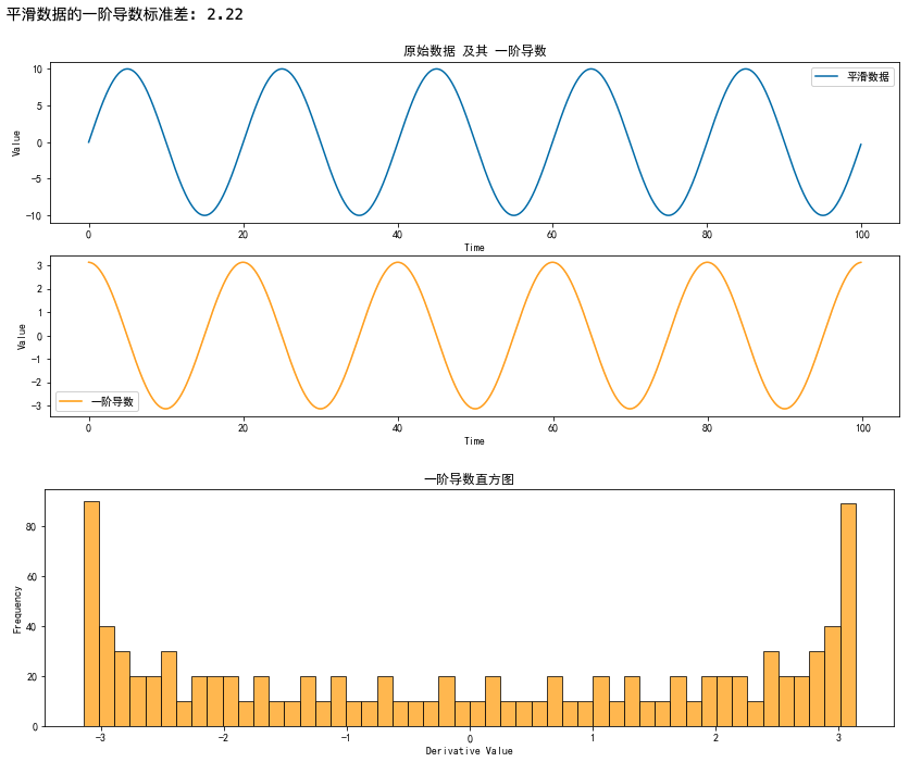
平滑曲線
import numpy as np
import matplotlib.pyplot as plt
from matplotlib import font_manager
fname="/usr/local/python3.6/lib/python3.6/site-packages/matplotlib/mpl-data/fonts/ttf/simhei.ttf"
zhfont = font_manager.FontProperties(fname=fname)


# 生成示例數據:正弦波加噪聲
np.random.seed(123456)
time = np.arange(0, 100, 0.1)
signal_period = 20  # 正弦波周期
signal = 10 * np.sin(2 * np.pi * time / signal_period)  # 正弦波

# 計算一階導數(離散形式)
dt = time[1] - time[0]  # 時間步長
first_derivative = np.diff(signal) / dt

# 計算一階導數的統計指標
std_dev_derivative = np.std(first_derivative)

# 打印導數的波動性指標
print(f"平滑數據的一階導數標準差: {std_dev_derivative:.2f}")

# 繪制原始信號與導數
plt.figure(figsize=(14, 6))

plt.subplot(2, 1, 1)
plt.plot(time, signal, label='平滑數據')
plt.xlabel('Time')
plt.ylabel('Value')
plt.title('原始數據 及其 一階導數', fontproperties=zhfont, fontsize=12)
plt.legend()

plt.subplot(2, 1, 2)
plt.plot(time[:-1], first_derivative, label='一階導數', color='orange')
plt.xlabel('Time')
plt.ylabel('Value')
# plt.title('原始數據求導', fontproperties=zhfont, fontsize=12)
plt.legend()
plt.show()

# 繪制導數的直方圖
plt.figure(figsize=(14, 4))
plt.hist(first_derivative, bins=50, color='orange', edgecolor='k', alpha=0.7)
plt.xlabel('Derivative Value')
plt.ylabel('Frequency')
plt.title('一階導數直方圖')
plt.show()
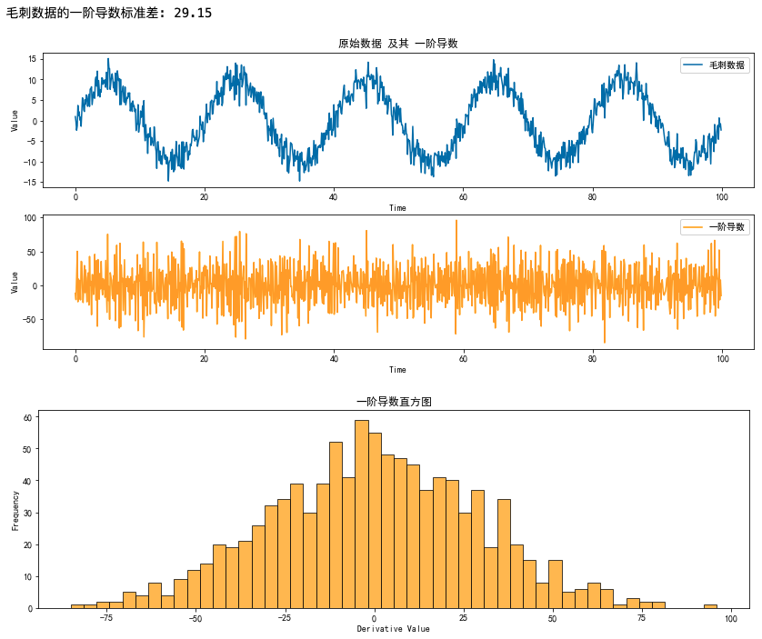
毛刺曲線
import numpy as np
import matplotlib.pyplot as plt
from matplotlib import font_manager
fname="/usr/local/python3.6/lib/python3.6/site-packages/matplotlib/mpl-data/fonts/ttf/simhei.ttf"
zhfont = font_manager.FontProperties(fname=fname)


# 生成示例數據:正弦波加噪聲
np.random.seed(123456)
time = np.arange(0, 100, 0.1)
signal_period = 20  # 正弦波周期
signal = 10 * np.sin(2 * np.pi * time / signal_period)  # 正弦波
noise = np.random.normal(0, 2, len(time))  # 噪聲
signal_with_noise = signal + noise

# 計算一階導數(離散形式)
dt = time[1] - time[0]  # 時間步長
first_derivative = np.diff(signal_with_noise) / dt

# 計算一階導數的統計指標
std_dev_derivative = np.std(first_derivative)

# 打印導數的波動性指標
print(f"毛刺數據的一階導數標準差: {std_dev_derivative:.2f}")

# 繪制原始信號與導數
plt.figure(figsize=(14, 6))

plt.subplot(2, 1, 1)
plt.plot(time, signal_with_noise, label='毛刺數據')
plt.xlabel('Time')
plt.ylabel('Value')
plt.title('原始數據 及其 一階導數', fontproperties=zhfont, fontsize=12)
plt.legend()

plt.subplot(2, 1, 2)
plt.plot(time[:-1], first_derivative, label='一階導數', color='orange')
plt.xlabel('Time')
plt.ylabel('Value')
# plt.title('原始數據求導', fontproperties=zhfont, fontsize=12)
plt.legend()
plt.show()

# 繪制導數的直方圖
plt.figure(figsize=(14, 4))
plt.hist(first_derivative, bins=50, color='orange', edgecolor='k', alpha=0.7)
plt.xlabel('Derivative Value')
plt.ylabel('Frequency')
plt.title('一階導數直方圖')
plt.show()
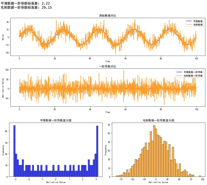
整體對比
import numpy as np
import matplotlib.pyplot as plt
from matplotlib import font_manager
fname="/usr/local/python3.6/lib/python3.6/site-packages/matplotlib/mpl-data/fonts/ttf/simhei.ttf"
zhfont = font_manager.FontProperties(fname=fname)


# 計算一階離散導數
dt = time[1] - time[0]
smooth_derivative = np.diff(signal) / dt
noisy_derivative = np.diff(signal_with_noise) / dt

# 計算標準差
std_dev_smooth = np.std(smooth_derivative)
std_dev_noisy = np.std(noisy_derivative)

# 打印結果
print(f"平滑數據一階導數標準差: {std_dev_smooth:.2f}")
print(f"毛刺數據一階導數標準差: {std_dev_noisy:.2f}")

# 繪制信號與導數
plt.figure(figsize=(12, 6))

plt.subplot(2, 1, 1)
plt.plot(time, smooth_signal, label='平滑數據', color='blue')
plt.plot(time, noisy_signal, label='毛刺數據', color='orange')
plt.xlabel('Time')
plt.ylabel('Value')
plt.title('原始數據對比', fontproperties=zhfont, fontsize=12)
plt.legend()

plt.subplot(2, 1, 2)
plt.plot(time[:-1], smooth_derivative, label='平滑數據一階導數', color='blue')
plt.plot(time[:-1], noisy_derivative, label='毛刺數據一階導數', color='orange')
plt.xlabel('Time')
plt.ylabel('Derivative Value')
plt.title('一階導數對比', fontproperties=zhfont, fontsize=12)
plt.legend()

plt.tight_layout()
plt.show()

# 繪制導數的直方圖
plt.figure(figsize=(12, 4))

plt.subplot(1, 2, 1)
plt.hist(smooth_derivative, bins=50, color='blue', edgecolor='k', alpha=0.7)
plt.xlabel('Derivative Value')
plt.ylabel('Frequency')
plt.title('平滑數據一階導數直方圖', fontproperties=zhfont, fontsize=12)

plt.subplot(1, 2, 2)
plt.hist(noisy_derivative, bins=50, color='orange', edgecolor='k', alpha=0.7)
plt.xlabel('Derivative Value')
plt.ylabel('Frequency')
plt.title('毛刺數據一階導數直方圖', fontproperties=zhfont, fontsize=12)

plt.tight_layout()
plt.show()
作者:Standby — 一生熱愛名山大川、草原沙漠,還有我們小郭寶貝!
出處:http://www.rzrgm.cn/standby/
本文版權歸作者和博客園共有,歡迎轉載,但未經作者同意必須保留此段聲明,且在文章頁面明顯位置給出原文連接,否則保留追究法律責任的權利。
出處:http://www.rzrgm.cn/standby/
本文版權歸作者和博客園共有,歡迎轉載,但未經作者同意必須保留此段聲明,且在文章頁面明顯位置給出原文連接,否則保留追究法律責任的權利。

 浙公網安備 33010602011771號