探秘Transformer系列之（31）--- Medusa

從零開始解析Transformer，目標是：(1) 解析Transformer如何運作，以及為何如此運作，讓新同學可以入門；(2) 力爭融入一些比較新的或者有特色的論文或者理念，讓老鳥也可以有所收獲。

探秘Transformer系列之（31）--- Medusa

0x00 概述

Medusa 是自投機領域較早的一篇工作，對后續工作啟發很大，其主要思想是multi-decoding head + tree attention + typical acceptance(threshold)。Medusa 沒有使用獨立的草稿模型，而是在原始模型的基礎上增加多個解碼頭（MEDUSA heads），并行預測多個后續 token。

正常的LLM只有一個用于預測t時刻token的head。Medusa 在 LLM 的最后一個 Transformer層之后保留原始的 LM Head，然后額外增加多個（假設是k個）可訓練的Medusa Head（解碼頭），分別負責預測t+1，t+2，...，和t+k時刻的不同位置的多個 Token。Medusa 讓每個頭生成多個候選 token，而非像投機解碼那樣只生成一個候選。然后將所有的候選結果組裝成多個候選序列，多個候選序列又構成一棵樹。再通過樹注意力機制并行驗證這些候選序列。

注：全部文章列表在這里，估計最終在35篇左右，后續每發一篇文章，會修改此文章列表。
cnblogs 探秘Transformer系列之文章列表

0x01 原理

1.1 動機

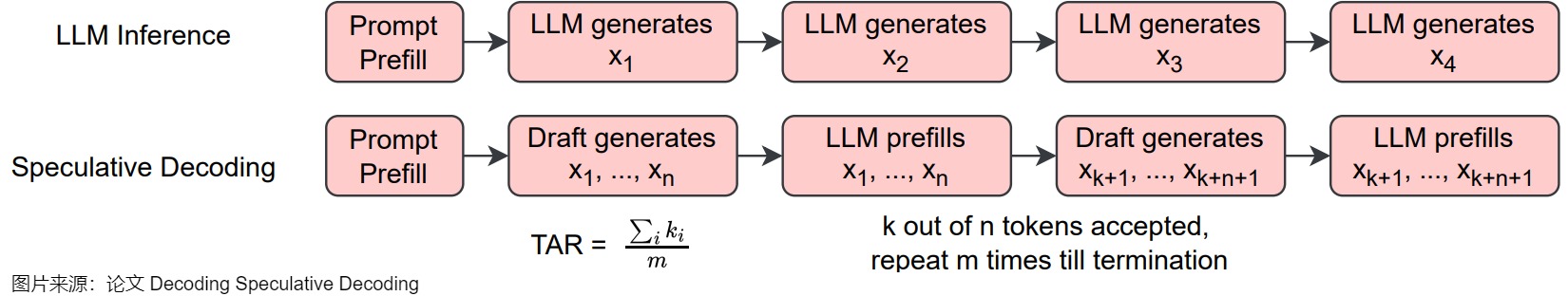
投機采樣的核心思路如上圖下方所示，首先以低成本的方式（一般來說是用小模型）快速生成多個候選 Token，然后通過一次并行驗證階段快速驗證多個 Token，進而減少大模型的 Decoding Step，實現加速的目的。然而，采用一個獨立的“推測”模型也有缺點，具體如下：

很難找到一個小而強的模型來生成對于原始的模型來說比較簡單的token。
- draft模型和大模型很難對齊，存在distribution shift。
- 并不是所有的LLM都能找到現成的小模型。重新訓練一個小模型需要較多的額外投入。
在一個系統中維護2個不同的模型，即增加了推理過程的計算復雜度，也導致架構上的復雜性，在分布式系統上的部署難度增大。
使用投機采樣的時候，會帶來額外的解碼開銷，尤其是當使用一個比較高的采樣溫度值時。

1.2 借鑒

Medua主要借鑒了兩個工作：BPD和SpecInfer。

大模型自身帶有一個LM head，用于把隱藏層輸出映射到詞表的概率分布，以實現單個token的解碼。為了生成多個token，論文“Blockwise Parallel Decoding for Deep Autoregressive Models”在骨干模型上使用多個解碼頭來加速推理，通過訓練輔助模型，使得模型能夠預測未來位置的輸出，然后利用這些預測結果來跳過部分貪心解碼步驟，從而加速解碼過程。
論文“SpecInfer: Accelerating Generative Large Language Model Serving with Speculative Inference and Token Tree Verification”的思路是：既然小模型可以猜測大模型的輸出并且效率非常高，那么一樣可以使用多個小模型來猜測多個 Token 序列，這樣提供的候選更多，猜對的機會也更大；為了提升這多個 Token 序列的驗證效率，作者提出 Token Tree Attention 的機制，首先將多個小模型生成的多個 Token 序列組合成 Token 樹，然后將其展開輸入模型，即可實現一次 decoding step 完成整個 Token 樹的驗證。

1.3 思路

基于這兩個思路來源，Medusa決定讓target LLM自己進行預測，即在target LLM最后一層decoder layer之上引入了多個額外的預測頭，使得模型可以在每個解碼步并行生成多個token，作為“推測”結果。我們進行具體分析。

1.3.1 單模型 & 多頭

為了拋棄獨立的 Draft Model，只保留一個模型，同時保留 Draft-then-Verify 范式，Medusa 在主干模型的最終隱藏層之后添加了若干個 Medusa Heads，每個解碼頭是一個帶殘差連接的單層前饋網絡。這些Medusa Heads是對BPD中多 Head 的升級，即由原來的一個 Head 生成一個 Token 變成一個 head 生成多個候選 Token。因為這些 Heads 具有預測對應位置 token 的能力，并且可以并行地執行，因此可以實現在一次前向中得到多個 draft tokens。具體如下圖所示。

可能有讀者會有疑問，后面幾個head要跨詞預測，其準確率應該很難保證吧？確實是這樣的，但是，如果我每個預測時間步都取top3出來，那么最終預測成功的概率就高不少了。而且，Medusa 作者觀察到，雖然在預測 next next Token 的時候 top1 的準確率可能只有 60%，但是如果選擇 top5，則準確率有可能超過 80%。而且，因為 MEDUSA 解碼頭與原始模型共享隱藏層狀態，所以分布差異較小。

1.3.2 Tree 驗證

因為貪心解碼的正確率不夠高，加速效果不夠顯著，因此Medusa讓每個Head解碼top-k個候選，不同head的候選集合組成一個樹狀結構。為了更高效地驗證這些 draft tokens，Medusa根據這些 Head 生成 Token 的笛卡爾積來構建出多個 Token 序列。然后使用Tree Attention方法，在注意力計算中，只允許同一延續中的 token 互相看到（attention mask），再加上位置編碼的配合，就可以在不增加 batch size 的情況下并行處理多個候選。

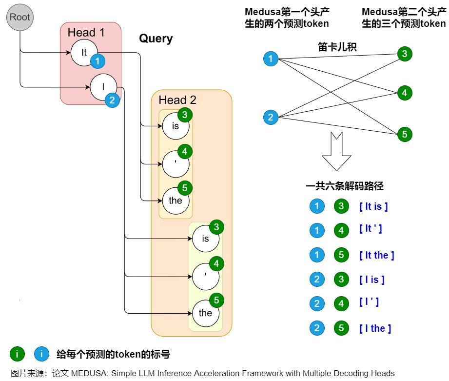
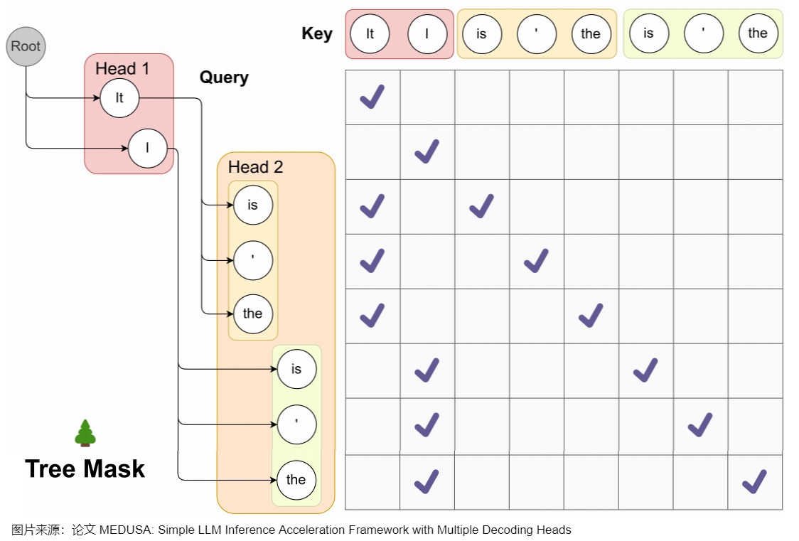
Medusa 中的樹和注意力掩碼矩陣如下圖所示。在每一跳中，我們看到圖中Medusa保留了多個可能的token，也就是概率最高的幾個token。這樣構成了所謂的樹結構，直觀來說，就是每1跳的每1個token都可能和下1跳的所有token組合成句子，也可以就在這1跳終止。例如，在圖中，一共2個head生成了2跳的token，那么這棵樹包含了6種可能的句子：Head 1 在下一個位置生成 2 個可能的 Token（It 和 I），Head 2 在下下一個位置生成 3 個可能的 Token（is，’ 和 the），這樣下一個位置和下下一個位置就有了 2 x 3 = 6 種可能的候選序列，如下圖左側所示。

而其對應的 Attention Mask 矩陣如右側所示。與原始投機解碼略有不同的地方是，樹中有多條解碼路徑，不同解碼路徑之間不能相互訪問。比如，(1) "It is"和 (2) "I is"是兩條路徑，那么在計算(1).is的概率分布時，只能看到(1).it，而不能看到(2)中的"I"。因此，Medusa新建了在并行計算多條路徑概率分布時需要的attention mask，稱為"Tree attention"。本質上就是同一條路徑內遵從因果mask的規則，不同路徑之間不能相互訪問。

Medusa作者稱，SpecInfer中每個speculator生成稱的序列長度不同，所以Mask是動態變化的。而Medusa的Tree Attention Mask在Infrence過程中是靜態不變的，這使得對樹注意力Mask的預處理進一步提高了效率。

1.3.3 小結

下表給出了BPD，SpecInfer，Medusa之間的差異。

領域	Blockwise Parallel Decoding	SpecInfer	Medusa
多模型	沒有真的構造出k-1個輔助模型，只對原始模型略作改造，讓其具備預測后k個token的能力	采用一批small speculative models（SSMs），并行預測多個候選SSM，可以是原始LLM的蒸餾、量化、剪枝版本
多頭	加入k個project layer，這k個project layer的輸出就是k個不同位置token的logits		在 LLM 的最后一個 Transformer Layer 之后保留原始的 LM Head，然后額外增加多個 Medusa Head，獲得多個候選的 Token 序列
Tree		將SSMs預測的多個候選merge為一個新的token tree，采用原始LLM做并行驗證。SpecInfer中每個speculator生成稱的序列長度不同，所以Mask是動態變化的。	Medusa的Tree Attention Mask在Infrence過程中是靜態不變的，這使得對樹注意力Mask的預處理進一步提高了效率。
訓練	重新訓練原始模型	訓練小模型	并不需要重新訓練整個大模型，而是凍結大模型而只訓練解碼頭

0x02 設計核心點

2.1 流程

MEDUSA的大致思路和投機解碼類似，其中每個解碼步驟主要由三個子步驟組成：

生成候選者。MEDUSA通過接在原模型的多個Medusa解碼頭來獲取多個位置的候選token
處理候選者。MEDUSA把各個位置的候選token進行處理，選出一些候選序列。然后通過tree attention來進行驗證。由于 MEDUSA 頭位于原始模型之上，因此，此處計算的 logits可以用于下一個解碼步驟。
接受候選者。通過typical acceptance（典型接受）來選擇最終輸出的結果。

Medusa更大的優勢在于，除了第一次Prefill外，后續可以達到邊verify邊生成的效果，即 Medusa 的推理流程可以理解：Prefill + Verify + Verify + ...。

2.2 模型結構

下面代碼給出了美杜莎的模型結構。Medusa 是在 LLM 的最后一個 Transformer Layer 之后保留原始的 LM Head，然后額外加多個 Medusa Head，也就是多個不同分支輸出。這樣可以預測出多個候選的 Token 序列。
Medusa head的輸入是大模型的隱藏層輸出。這是和使用外掛小模型投機解碼的另一個重要不同。外掛小模型的輸入是查表得到的token embedding，比這里的大模型最后一層隱藏層要弱的多，因此比較依賴小模型的性能。正是因為借助大模型的隱藏層輸出，這里的Medusa head的結構都十分簡單。

class MedusaLlamaModel(KVLlamaForCausalLM):
    """The Medusa Language Model Head.
    This module creates a series of prediction heads (based on the 'medusa' parameter)
    on top of a given base model. Each head is composed of a sequence of residual blocks
    followed by a linear layer.
    """

    def __init__(
        self,
        config,
    ):
        # Load the base model
        super().__init__(config)
        # For compatibility with the old APIs

        medusa_num_heads = config.medusa_num_heads
        medusa_num_layers = config.medusa_num_layers
        base_model_name_or_path = config._name_or_path
        self.hidden_size = config.hidden_size
        self.vocab_size = config.vocab_size
        self.medusa = medusa_num_heads
        self.medusa_num_layers = medusa_num_layers
        self.base_model_name_or_path = base_model_name_or_path
        self.tokenizer = AutoTokenizer.from_pretrained(self.base_model_name_or_path)
        # Create a list of Medusa heads
        self.medusa_head = nn.ModuleList(
            [
                nn.Sequential(
                    *([ResBlock(self.hidden_size)] * medusa_num_layers),
                    nn.Linear(self.hidden_size, self.vocab_size, bias=False),
                )
                for _ in range(medusa_num_heads)
            ]
        )
        

    def forward(
        self,
        input_ids=None,
        attention_mask=None,
        past_key_values=None,
        output_orig=False,
        position_ids=None,
        medusa_forward=False,
        **kwargs,
    ):
        """Forward pass of the MedusaModel.

        Args:
            input_ids (torch.Tensor, optional): Input token IDs.
            attention_mask (torch.Tensor, optional): Attention mask.
            labels (torch.Tensor, optional): Ground truth labels for loss computation.
            past_key_values (tuple, optional): Tuple containing past key and value states for attention.
            output_orig (bool, optional): Whether to also output predictions from the original LM head.
            position_ids (torch.Tensor, optional): Position IDs.

        Returns:
            torch.Tensor: A tensor containing predictions from all Medusa heads.
            (Optional) Original predictions from the base model's LM head.
        """
        if not medusa_forward:
            return super().forward(
                input_ids=input_ids,
                attention_mask=attention_mask,
                past_key_values=past_key_values,
                position_ids=position_ids,
                **kwargs,
            )
        with torch.inference_mode():
            # Pass input through the base model
            outputs = self.base_model.model(
                input_ids=input_ids,
                attention_mask=attention_mask,
                past_key_values=past_key_values,
                position_ids=position_ids,
                **kwargs,
            )
            if output_orig:
                # 原始模型輸出
                orig = self.base_model.lm_head(outputs[0])
        # Clone the output hidden states
        hidden_states = outputs[0].clone()
        medusa_logits = []
        # TODO: Consider parallelizing this loop for efficiency?
        for i in range(self.medusa):
            # 美杜莎頭輸出
            medusa_logits.append(self.medusa_head[i](hidden_states))
        if output_orig:
            return torch.stack(medusa_logits, dim=0), outputs, orig
        return torch.stack(medusa_logits, dim=0)

2.3 多頭

2.3.1 head結構

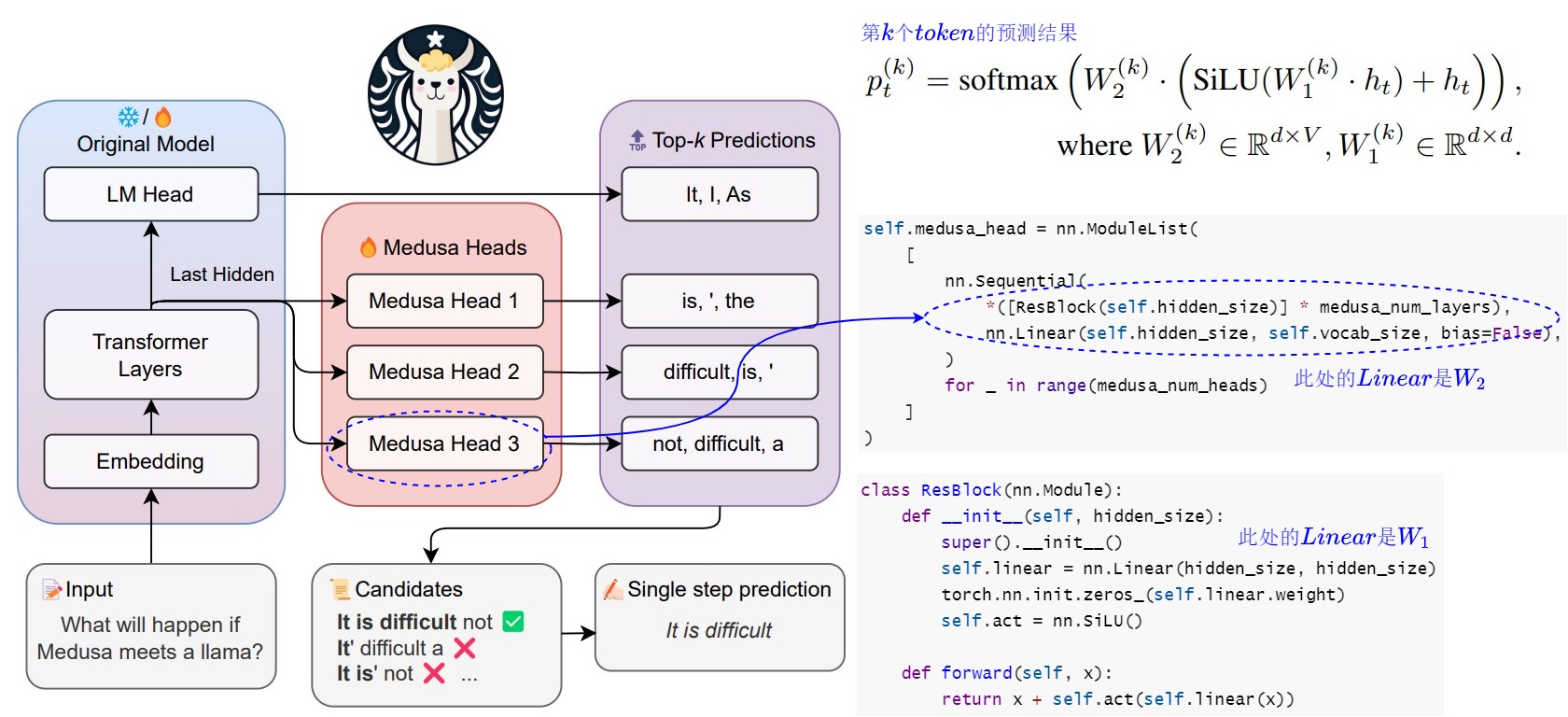
Medusa 額外新增 medusa_num_heads 個 Medusa Head，每個 Medusa Head 是一個加上了殘差連接的單層前饋網絡，其中的 Linear 和模型的默認 lm_head 維度一樣，這樣可以預測后續的 Token。

self.medusa_head = nn.ModuleList(
    [
        nn.Sequential(
            *([ResBlock(self.hidden_size)] * medusa_num_layers),
            nn.Linear(self.hidden_size, self.vocab_size, bias=False),
        )
        for _ in range(medusa_num_heads)
    ]
)

下面代碼為打印出來的實際內容。

ModuleList(
  (0-3): 4 x Sequential(
    (0): ResBlock(
      (linear): Linear(in_features=4096, out_features=4096, bias=True)
      (act): SiLU()
    )
    (1): Linear(in_features=4096, out_features=32000, bias=False)
  )
)

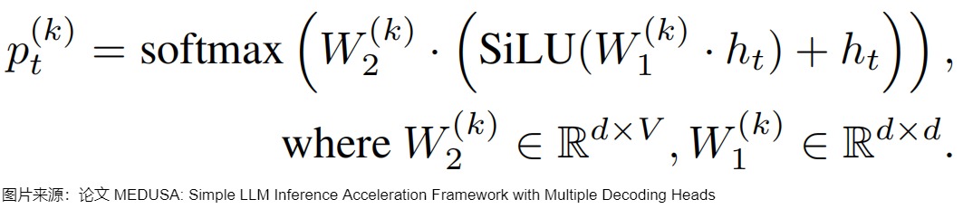
把第k個解碼頭在詞表上的輸出分布記作 $p_t^{(t)}$，其計算方式如下。d是hidden state的輸出維度，V是詞表大小，原始模型的預測表示為 $p_t^{(0)}$ 。

下面是把代碼和模型結構結合起來的示意圖。

2.3.2 位置

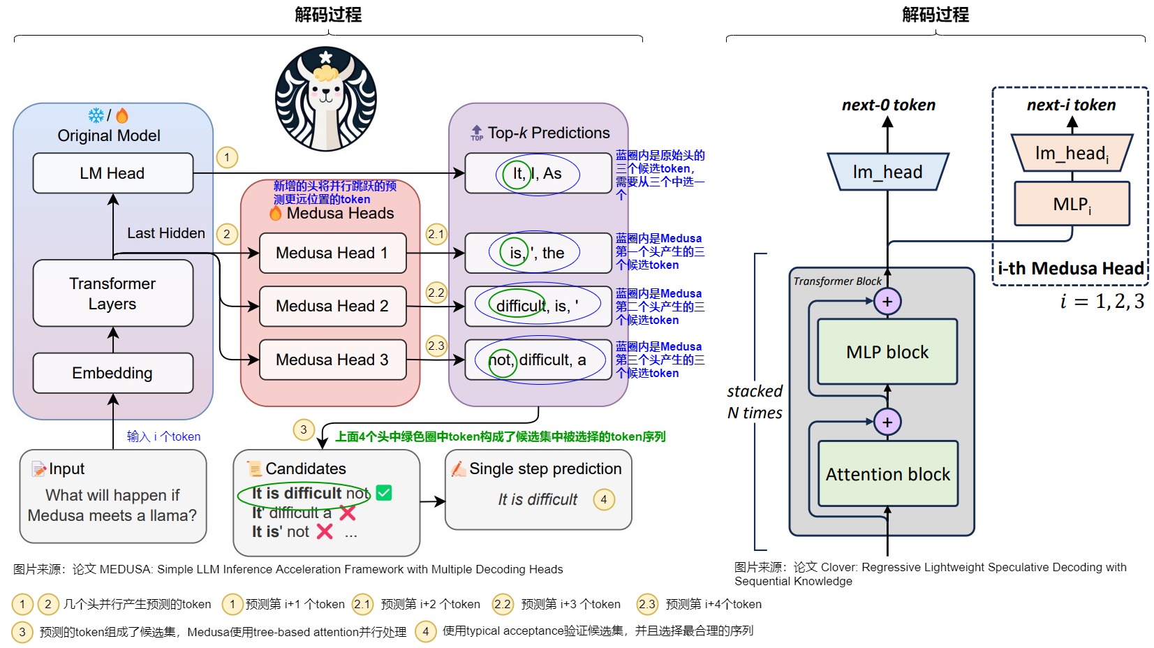
Medusa每個頭預測的偏移量是不同的，第k個頭用來預測位置t+k+1的輸出token（k的取值是1~K）。原模型的解碼頭依然預測位置t+1的輸出，相當于k=0。具體而言，把原始模型在位置t的最后隱藏狀態 $?_t$接入到K個解碼頭上，對于輸入token序列 $t_0,t_1,..,t_i$，原始的head根據輸入預測$ t_{i+1}$，Medusa新增的第一個head根據輸入預測 $t_{i+2}$的token，也就是跳過token $t_{i+1}$ 預測下一個未來的token。并且每個頭可以指定topk個結果。這些頭的預測結果構成了多個候選詞匯序列，然后利用樹形注意力機制同時處理這些候選序列。在每個解碼步，選擇最長被接受的候選序列作為最終的預測結果。這樣，每步可以預測多個詞匯，從而減少了總的解碼步數，提高了推理速度。

如下圖所示，Medusa在原始模型基礎上，增加了3個額外的Head，可以并行預測出后4個token的候選。

2.4 缺點

Medusa的缺點如下：

Medusa 新增的 lm_head 和最后一個 Transformer Block 中間只有一個 MLP，表達能力可能有限。
Medusa 增加了模型參數量，會增加顯存占用；
Medusa 每個 head 都是獨立執行的，也就是 “next next token” 預測并不會依賴上一個 “next token” 的結果，導致生成效果不佳，接受率比較低，在大 batch size 時甚至可能負優化。
缺乏序列依賴也可能導致低效的樹剪枝算法。
草稿質量仍然不高，加速效果有限，并且在非貪婪解碼 (non-greedy decoding) 下不能保證輸出分布與目標LLM一致。

因此，后續有研究工作對此進行了改進。比如Clover重點是提供序列依賴和加入比單個 MLP 具有更強的表征能力的模塊。Hydra 增加了 draft head 預測之間的關聯性。Hydra++使用 base model 的輸出預測概率作為知識蒸餾的教師模型輸出來訓練 draft head。并且類似EAGLE，Hydra++增加一個獨立的 decoder layer，每個 Hydra head 除了上一個 token 本身，還添加了上一個 token 在這個 decoder layer 的 representation 作為輸入。

0x03 Tree Verification

每個Medusa Head 會生成 top-k 個預測標記，然后通過計算這些預測的笛卡爾積來形成候選序列。我們可以對于每個候選序列都走一遍模型來驗證，但是這樣做太耗時。因此，Medusa 作者設計了一種tree attention的機制，在候選樹內進行掩碼操作，掩碼限制某個token對前面token的注意力。同時，也要為相應地為position embedding設置正確的位置索引。因為有 tree attention 的存在，所以 Medusa 可以并行地構建、維護和驗證多個候選序列。

3.1 解碼路徑

在Medusa中，基礎版本解碼采用greedy方式取Top-1 Token。Medusa增加額外的解碼頭之后，使用 Top-K Sampling，每一個 Head 都會輸出 k 個 tokens。不同Medusa頭之間預測結果不一致。$p(t_{t+1}|t_0,...,t_i)$和$p(t_{t+2}|t_0,...,t_i)$形式上是條件獨立的，但是實際上$p_{t+2}$依賴$p_{t+1}$，不能直接取$p(t_{t+1}|t_0,...,t_i)$和$p(t_{t+2}|t_0,...,t_i)$最大的token作為verify階段的輸入，這樣組成的句子可能會在邏輯上不一致。因此，Medusa還引入采樣topk組合作為候選序列的方式去緩解這個問題。最終把LM_head 的輸出作為根節點構建出樹狀結構，樹的深度自頂向下遍歷稱為解碼路徑（論文中叫做candidates path）。每個候選序列可以表示所構建的tree上的一條路徑上所有的node（而不只是leaf node，因為tree attention驗證的時候會把路徑上所有token都進行驗證）。

由于有K個head，每個head選取$\text{top-}s_k$個預測輸出，則所有路徑可能組合為樹上所有節點的總和，即$\sum_{k=1}^K \prod_{i=1}^k s_i$。在構建樹形結構時，最簡單的方法是通過笛卡爾積來獲取多個解碼頭組成的所有可能的候選序列。下圖例子使用了Cartesian product對兩個解碼頭的結果進行處理，獲得所有候選序列。具體來說就是將每個頭的top-k個詞作為節點，每個頭作為樹的一層。圖上一共存在6條解碼路徑，相當于 Head 1 在下一個位置生成 2 個可能的 Token（It 和 I），Head 2 在下下一個位置生成 3 個可能的 Token（is，’ 和 the），這樣下一個位置和下下一個位置就有了 2 x 3 = 6 種可能的候選序列。為了區分不同的 prefix，Medusa 設置了一些冗余，例如 Head 2 的三個預測 token 均出現了兩次，這是為了分別對應 It 和 I 這兩個不同的 prefix。每個 token 在 tree mask 的作用下只可以看見自己的 prefix。

3.2 最佳構造方式

上圖采用top-3，兩個頭一共有6條候選路徑。如果解碼頭數量數量比較多，每個頭給出的候選token也比較多。解碼路徑會隨著Top-k 和頭數增多急劇增加，會產生大量的候選路徑，具有龐大的搜索空間。雖然增加候選序列的數量，最終接受token的命中率就會提升，但是驗證更多候選序列也會帶來額外的計算消耗。那么新的問題是：

如何能減少候選解碼路徑？
如何能在候選解碼路徑中，得到最優解碼路徑？

直觀上來說，那些由不同頭部的topk預測組成的候選結果可能具有不同的準確率。應該優先選擇那些更準確的預測，從而構建一個更有效的樹，而不需要使用所有可能的排列組合。Medusa 通過在校準數據集上統計每個解碼頭的 top-k 預測的準確率，然后貪婪地選擇那些能夠最大化期望接受長度的節點，將它們加入到樹中。這樣可以在相同的節點總數下，獲得更高的加速比。其實，此方法本質上就是用剪枝來加速，剪去每個head中$\text{top-}s_k$的若干個。

具體來說，我們可以使用一個calibration dataset（比如Alpaca-eval dataset）來獲取不同解碼頭給出的各個token的準確率：把第 k 個解碼頭給出的第 i 個token的準確率記為 $a_k^{(i)}$。假設各個token的準確率之間是獨立的，那么一個由$[i_1,i_2,\cdots,i_k] $構成的候選序列的準確率可以寫作 $\prod_{j=1}^ka_j^{(i_j)}$。我們用 I 表示候選序列的集合，那么集合里的候選序列的expectation of acceptance length就表示為：

\[\sum_{[i_1,i_2,\cdots,i_k]\in I}\prod_{j=1}^ka_j^{(i_j)} \]

在構建tree的時候，Medusa 用貪心算法優先加入當前有最大準確率的候選序列，直到tree的節點數量達到接受長度的期望值上限，這樣能最大化expectation of acceptance length，也就能最大化acceleration rate。這是一種手工設計的稀疏樹結構，越靠前的節點，有更多的子節點路徑。即，把所有位置組合窮舉，然后選取前??個組合作為固定考察的可能，剩余的剪枝去掉。

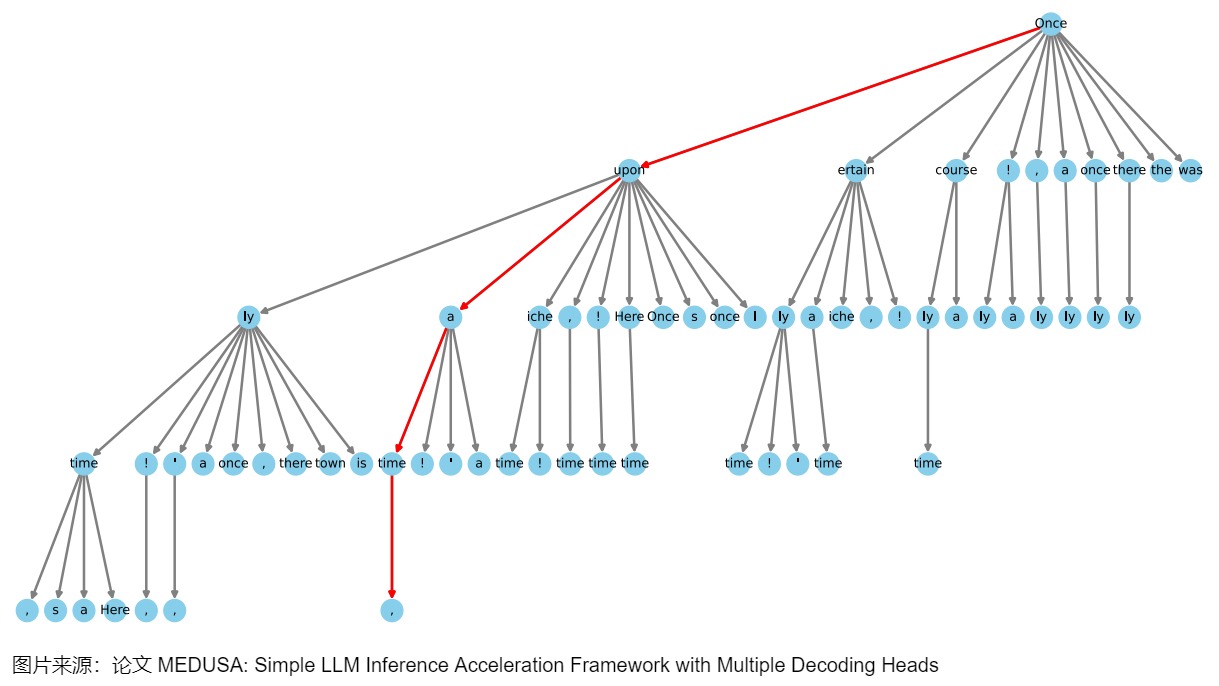
MEDUSA-2 Vicuna-7B模型的一個稀疏樹示例如下圖所示。這個樹結構延伸了四個層次，表明有四個MEDUSA頭參與了計算。該樹最初通過笛卡爾積方法生成，隨后根據每個MEDUSA頭在Alpaca-eval數據集上測量的前 k 個預測的統計期望值進行修剪。樹向左傾斜在視覺上代表了算法傾向于使用更高準確率的token，每個節點表示MEDUSA頭部的top-k預測中的一個token，邊顯示了它們之間的連接，紅線突出顯示了正確預測未來token的路徑。這樣就將1000個路徑的樹優化到只有42條路徑，而且，這里的路徑可以提前結束，不要求一定要遍歷到最后一層。

3.3 實現

3.3.1 關鍵變量

我們首先看看注意力樹所涉及的關鍵變量。

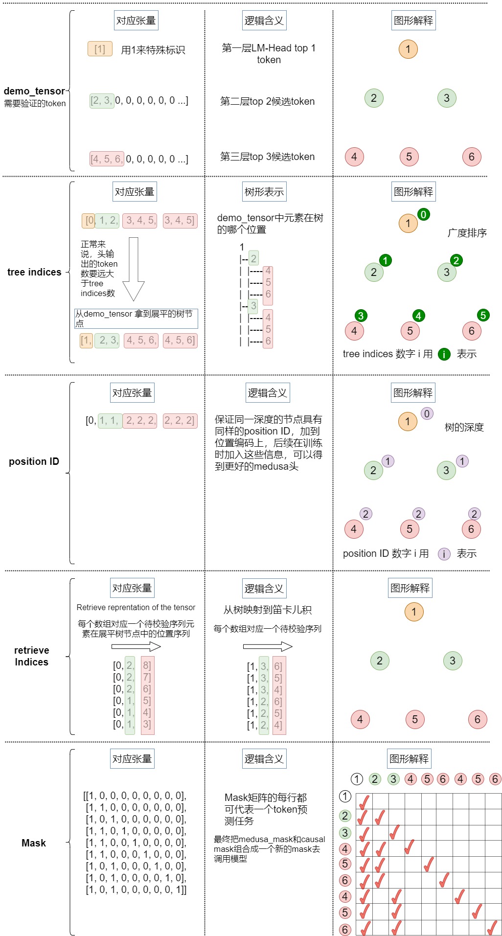
demo_tensor

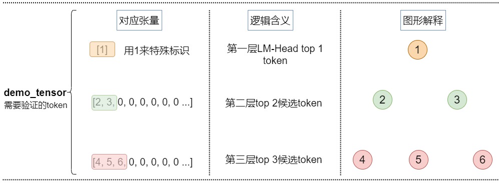
demo_tensor是輸入張量，例子如下：

[2, 3, 0, 0, 0, 0, 0, 0 ...] # 1st depth we choose top 2
[4, 5, 6, 0, 0, 0, 0, 0 ...] # 2nd depth we choose top 3

對應下圖。

medusa_choices

medusa_choices是一個嵌套列表，表示medusa樹結構，決定解碼路徑。外部列表對應于樹中的節點，每個內部列表給出該節點在樹中的祖先及其位置。根據Medusa choies 我們可以構建稀疏樹的所有數據成員，源碼中的例子如下。

vicuna_7b_stage2 = [(0,), (0, 0), (1,), (0, 1), (0, 0, 0), (1, 0), (2,), (0, 2), (0, 0, 1), (0, 3), (3,), (0, 1, 0), (2, 0), (4,), (0, 0, 2), (0, 4), (1, 1), (1, 0, 0), (0, 0, 0, 0), (5,), (0, 0, 3), (0, 5), (0, 2, 0), (3, 0), (0, 1, 1), (0, 6), (6,), (0, 7), (0, 0, 4), (4, 0), (1, 2), (0, 8), (7,), (0, 3, 0), (0, 0, 0, 1), (0, 0, 5), (2, 1), (0, 0, 6), (1, 0, 1), (0, 0, 1, 0), (2, 0, 0), (5, 0), (0, 9), (0, 1, 2), (8,), (0, 4, 0), (0, 2, 1), (1, 3), (0, 0, 7), (0, 0, 0, 2), (0, 0, 8), (1, 1, 0), (0, 1, 0, 0), (6, 0), (9,), (0, 1, 3), (0, 0, 0, 3), (1, 0, 2), (0, 5, 0), (3, 1), (0, 0, 2, 0), (7, 0), (1, 4)]
vicuna_7b_stage1_ablation = [(0,), (0, 0), (1,), (0, 0, 0), (0, 1), (1, 0), (2,), (0, 2), (0, 0, 1), (3,), (0, 3), (0, 1, 0), (2, 0), (0, 0, 2), (0, 4), (4,), (0, 0, 0, 0), (1, 0, 0), (1, 1), (0, 0, 3), (0, 2, 0), (0, 5), (5,), (3, 0), (0, 1, 1), (0, 6), (6,), (0, 0, 4), (1, 2), (0, 0, 0, 1), (4, 0), (0, 0, 5), (0, 7), (0, 8), (0, 3, 0), (0, 0, 1, 0), (1, 0, 1), (7,), (2, 0, 0), (0, 0, 6), (2, 1), (0, 1, 2), (5, 0), (0, 2, 1), (0, 9), (0, 0, 0, 2), (0, 4, 0), (8,), (1, 3), (0, 0, 7), (0, 1, 0, 0), (1, 1, 0), (6, 0), (9,), (0, 0, 8), (0, 0, 9), (0, 5, 0), (0, 0, 2, 0), (1, 0, 2), (0, 1, 3), (0, 0, 0, 3), (3, 0, 0), (3, 1)]
vicuna_7b_stage1 = [(0,), (0, 0), (1,), (2,), (0, 1), (1, 0), (3,), (0, 2), (4,), (0, 0, 0), (0, 3), (5,), (2, 0), (0, 4), (6,), (0, 5), (1, 1), (0, 0, 1), (7,), (3, 0), (0, 6), (8,), (9,), (0, 1, 0), (0, 7), (0, 8), (4, 0), (0, 0, 2), (1, 2), (0, 9), (2, 1), (5, 0), (1, 0, 0), (0, 0, 3), (1, 3), (0, 2, 0), (0, 1, 1), (0, 0, 4), (6, 0), (1, 4), (0, 0, 5), (2, 2), (0, 3, 0), (3, 1), (0, 0, 6), (7, 0), (1, 5), (1, 0, 1), (2, 0, 0), (0, 0, 7), (8, 0), (0, 0, 0, 0), (4, 1), (0, 1, 2), (0, 4, 0), (9, 0), (0, 2, 1), (2, 3), (1, 6), (0, 0, 8), (0, 5, 0), (3, 2), (5, 1)]

我們此處例子為：[[0], [0, 0], [0, 1], [0, 2], [1], [1, 0], [1, 1], [1, 2]]，這里[1]為根節點，則可視化如下。

[1]
[2, 3]
[4, 5, 6]

medusa_buffers

medusa_buffers數據結構信息如下。

medusa_buffers = generate_medusa_buffers(medusa_choices, device='cpu')

medusa_buffers = {
    "medusa_attn_mask": medusa_attn_mask.unsqueeze(0).unsqueeze(0),
    "tree_indices": medusa_tree_indices,
    "medusa_position_ids": medusa_position_ids,
    "retrieve_indices": retrieve_indices,
    }

其中成員變量作用如下：

medusa_attn_mask：就是樹注意力用到的掩碼。
tree_indices：demo_tensor中元素在樹的哪個位置，在 generate_candidates()函數中會用到。
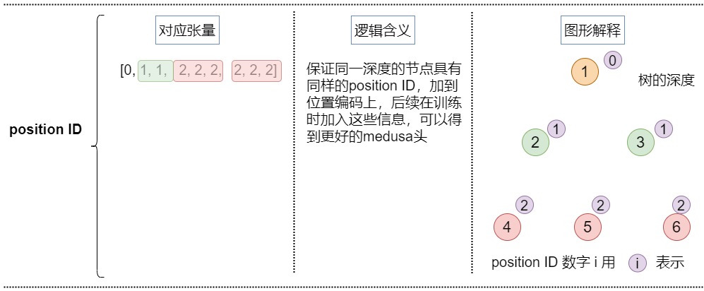
medusa_position_ids：保證同一深度的節點具有同樣的position ID，加到位置編碼上，后續在訓練時加入這些信息，可以得到更好的medusa頭。在tree_decoding()函數中用到。
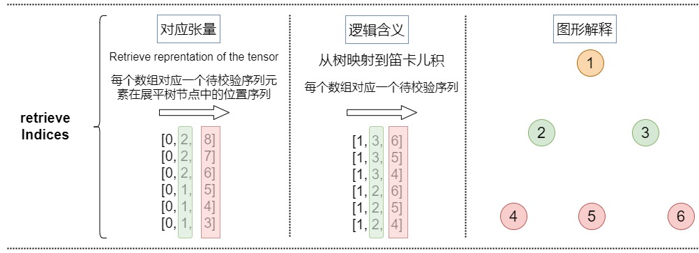
retrieve_indices：從樹映射到笛卡爾積，代表每個笛卡爾積在logits中的位置。依據這些信息，可以從logits里面提取每個笛卡爾積對應的logits。在tree_decoding()函數和generate_candidates()函數中用到。

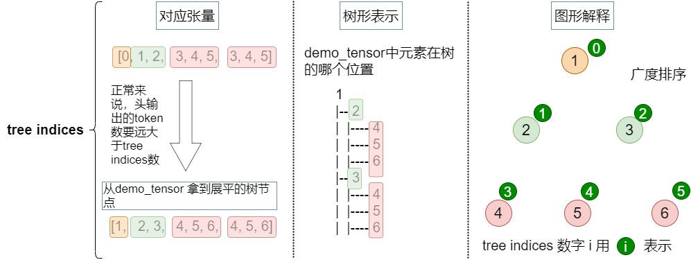
tree_indices

tree_indices代表demo_tensor中元素在樹的哪個位置。對于給定的輸入張量，對應的tree_indices如下。

[0, 1, 2, 3, 4, 5, 3, 4, 5]

長成的樹如下。

1
|-- 2
|  |-- 4
|  |-- 5
|  |-- 6
|-- 3
|  |-- 4
|  |-- 5
|  |-- 6

從demo_tensor 拿到展平的樹節點如下。

[1, 2, 3, 4, 5, 6, 4, 5, 6]

參見下圖。

medusa_position_ids

medusa_position_ids：保證同一深度的節點具有同樣的position ID。加入這些信息之后，每個token對應的位置編碼是：序列中的位置 + 樹中的深度。這樣在后續訓練medusa頭時就知道深度信息，可以訓練出更好的medusa頭。在tree_decoding()函數中用到此變量。

輸入張量對應的位置id如下。

[0, 1, 1, 2, 2, 2, 2, 2, 2] # Medusa position IDs
 |  |  |  |  |  |  |  |  |
[1, 2, 3, 4, 5, 6, 4, 5, 6] # Flatten tree representation of the tensor

可視化如下。

retrieve_indices

retrieve_indices是從樹映射到笛卡爾積，代表每個笛卡爾積在logits中的位置。依據這些信息，可以從logits里面提取每個笛卡爾積對應的logits。

本例的retrieve_indices如下。

[0, 2, 8]
[0, 2, 7]
[0, 2, 6]
[0, 1, 5]
[0, 1, 4]
[0, 1, 3]

把樹映射到笛卡爾積之后如下。

[1, 3, 6]
[1, 3, 5]
[1, 3, 4]
[1, 2, 6]
[1, 2, 5]
[1, 2, 4]

具體可視化如下。

medusa_attn_mask

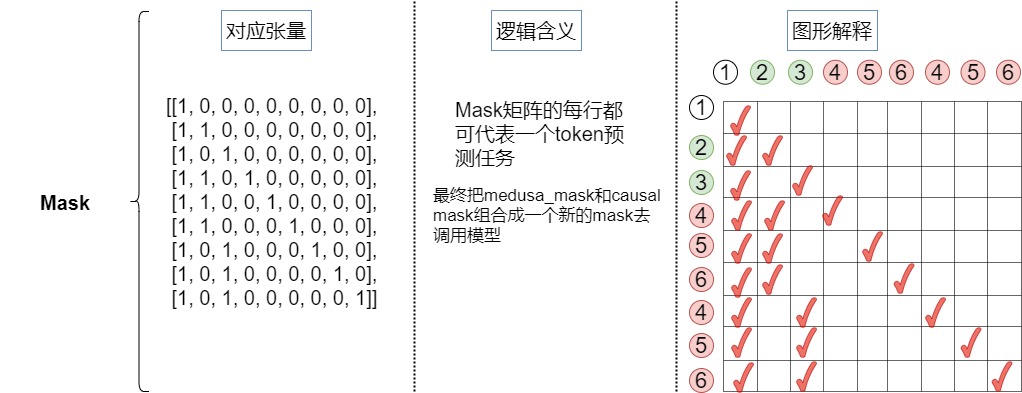
因為最終組成的樹是將每個頭的top-k個詞作為節點，每個頭作為樹的一層，每條直到葉子節點的路徑構成一組待驗證的預測。在這棵樹內，Attention Mask需要新的設計，該Mask只限制一個token對前面token的注意力。同時，要為相應地為position embedding設置正確的位置索引。掩碼矩陣的細節如下：

Mask矩陣的每行都可以代表一個token預測任務
在Tree Mask矩陣中，需要對位置編碼進行錯位編碼

論文中例子如下。

對于本例的掩碼如下。

3.3.2 示例代碼

示例代碼如下

demo_tensor = torch.zeros(2,10).long()
demo_tensor[0,0] = 2
demo_tensor[0,1] = 3
demo_tensor[1,0] = 4
demo_tensor[1,1] = 5
demo_tensor[1,2] = 6
print('Demo tensor: \n', demo_tensor)
demo_tensor = demo_tensor.flatten()
demo_tensor = torch.cat([torch.ones(1).long(), demo_tensor])
print('='*50)
medusa_choices = [[0], [0, 0], [0, 1], [0, 2], [1], [1, 0], [1, 1], [1, 2]]
medusa_buffers = generate_medusa_buffers(medusa_choices, device='cpu')
tree_indices = medusa_buffers['tree_indices']
medusa_position_ids = medusa_buffers['medusa_position_ids']
retrieve_indices = medusa_buffers['retrieve_indices']
print('Tree indices: \n', tree_indices.tolist())
print('Tree reprentation of the tensor: \n', demo_tensor[tree_indices].tolist())
print('='*50)
print('Medusa position ids: \n', medusa_position_ids.tolist())
print('='*50)
print('Retrieve indices: \n', retrieve_indices.tolist())
demo_tensor_tree = demo_tensor[tree_indices]
demo_tensor_tree_ext = torch.cat([demo_tensor_tree, torch.ones(1).long().mul(-1)])
print('Retrieve reprentation of the tensor: \n', demo_tensor_tree_ext[retrieve_indices].tolist())
print('='*50)
demo_tensor_tree_ext[retrieve_indices].tolist()
print('='*50)
print(medusa_buffers['medusa_attn_mask'][0,0,:,:].int())
print('='*50)
print(medusa_buffers['medusa_attn_mask'][0,0,:,:].int())

打印結果：

Demo tensor: 
 tensor([[2, 3, 0, 0, 0, 0, 0, 0, 0, 0],
        [4, 5, 6, 0, 0, 0, 0, 0, 0, 0]])
==================================================
Tree indices: 
 [0, 1, 2, 11, 12, 13, 11, 12, 13]
Tree reprentation of the tensor: 
 [1, 2, 3, 4, 5, 6, 4, 5, 6]
==================================================
Medusa position ids: 
 [0, 1, 1, 2, 2, 2, 2, 2, 2]
==================================================
Retrieve indices: 
 [[0, 2, 8], [0, 2, 7], [0, 2, 6], [0, 1, 5], [0, 1, 4], [0, 1, 3]]
Retrieve reprentation of the tensor: 
 [[1, 3, 6], [1, 3, 5], [1, 3, 4], [1, 2, 6], [1, 2, 5], [1, 2, 4]]
==================================================
tensor([[1, 0, 0, 0, 0, 0, 0, 0, 0],
        [1, 1, 0, 0, 0, 0, 0, 0, 0],
        [1, 0, 1, 0, 0, 0, 0, 0, 0],
        [1, 1, 0, 1, 0, 0, 0, 0, 0],
        [1, 1, 0, 0, 1, 0, 0, 0, 0],
        [1, 1, 0, 0, 0, 1, 0, 0, 0],
        [1, 0, 1, 0, 0, 0, 1, 0, 0],
        [1, 0, 1, 0, 0, 0, 0, 1, 0],
        [1, 0, 1, 0, 0, 0, 0, 0, 1]], dtype=torch.int32)

3.3.3 總體可視化

具體可視化參見下圖。

3.3.4 使用

調用

整體調用代碼如下。基本邏輯是：

根據設定的medusa choices得到稀疏的樹結構表達，具體涉及generate_medusa_buffers()函數。
初始化key和value。
構建樹注意力掩碼，根據輸入的 Prompt 進行預測，輸出 logits 和 medusa_logits。具體涉及initialize_medusa()函數。logits對應 lm_head 的輸出，medusa_logits對應medusa_head 的輸出。
從樹中提取用美杜莎頭得到的topk預測。這些預測構成了候選路徑。具體涉及generate_candidates()函數。
用樹注意力驗證候選路徑，得到最佳路徑。具體涉及tree_decoding()函數和evaluate_posterior()函數。tree_decoding()函數執行基于樹注意力（tree-attention-based）的推理。evaluate_posterior()函數執行對樹的驗證。
根據候選 Token 序列選出對應的 logits，medusa_logits，并更新輸入，key、value cache 等。具體涉及update_inference_inputs()函數。

def medusa_forward(input_ids, model, tokenizer, medusa_choices, temperature, posterior_threshold, posterior_alpha, top_p=0.8, sampling = 'typical', fast = True, max_steps = 512):

    # Avoid modifying the input_ids in-place
    input_ids = input_ids.clone()

    # Cache medusa buffers (the fixed patterns for tree attention)
    if hasattr(model, "medusa_choices") and model.medusa_choices == medusa_choices:
        # Load the cached medusa buffer
        medusa_buffers = model.medusa_buffers
    else:
        # Initialize the medusa buffer
        # 1. 根據設定的medusa choices得到稀疏的樹結構表達
        medusa_buffers = generate_medusa_buffers(
            medusa_choices, device=model.base_model.device
        )
    model.medusa_buffers = medusa_buffers
    model.medusa_choices = medusa_choices

    # Initialize the past key and value states
    if hasattr(model, "past_key_values"):
        past_key_values = model.past_key_values
        past_key_values_data = model.past_key_values_data
        current_length_data = model.current_length_data
        # Reset the past key and value states
        current_length_data.zero_()
    else:
        (
            past_key_values,
            past_key_values_data,
            current_length_data,
        ) = initialize_past_key_values(model.base_model)
        model.past_key_values = past_key_values
        model.past_key_values_data = past_key_values_data
        model.current_length_data = current_length_data

    input_len = input_ids.shape[1]
    reset_medusa_mode(model)
    
    # Initialize tree attention mask and process prefill tokens
    medusa_logits, logits = initialize_medusa(
            input_ids, model, medusa_buffers["medusa_attn_mask"], past_key_values
    )
    new_token = 0
    
    for idx in range(max_steps): 
        # Generate candidates with topk predictions from Medusa heads
        # 用美杜莎頭得到的topk預測來生成候選路徑。candidates是多個候選 Token 序列。tree_candidates是Token 樹
        candidates, tree_candidates = generate_candidates(
                medusa_logits,
                logits,
                medusa_buffers["tree_indices"],
                medusa_buffers["retrieve_indices"],
                temperature, posterior_threshold, posterior_alpha, top_p, sampling, fast
            )
        # Use tree attention to verify the candidates and get predictions
        # 用樹注意力驗證候選路徑。使用 Tree Attention 機制對 tree_candidates 進行驗證推理，獲得新的 logits 和 medusa_logits 輸出。
        medusa_logits, logits, outputs = tree_decoding(
                model,
                tree_candidates,
                past_key_values,
                medusa_buffers["medusa_position_ids"],
                input_ids,
                medusa_buffers["retrieve_indices"],
            )
        # 評估每條路徑合理性，得到最佳路徑。如果所有序列都沒有通過，則只使用第一個 Token，對應 accept_length 為 0，如果某個序列通過，則使用該序列中的已接受的 Token
        best_candidate, accept_length = evaluate_posterior(
                logits, candidates, temperature, posterior_threshold, posterior_alpha , top_p, sampling, fast
            )
        # 根據候選 Token 序列選出對應的 logits，medusa_logits，并更新輸入，key、value cache 等
        input_ids, logits, medusa_logits, new_token = update_inference_inputs(
                input_ids,
                candidates,
                best_candidate,
                accept_length,
                medusa_buffers["retrieve_indices"],
                outputs,
                logits,
                medusa_logits,
                new_token,
                past_key_values_data,
                current_length_data,
            )
        if tokenizer.eos_token_id in input_ids[0, input_len:].tolist():
            break
        if new_token > 1024:
            break
    return input_ids, new_token, idx

初始化

initialize_medusa()函數會進行初始化操作，得到logits和mask。

def initialize_medusa(input_ids, model, medusa_attn_mask, past_key_values):
    """
    Initializes the Medusa structure for a given model.

    This function performs the following operations:
    1. Forward pass through the model to obtain the Medusa logits, original model outputs, and logits.
    2. Sets the Medusa attention mask within the base model.

    Args:
    - input_ids (torch.Tensor): The input tensor containing token ids.
    - model (MedusaLMHead): The model containing the Medusa layers and base model.
    - medusa_attn_mask (torch.Tensor): The attention mask designed specifically for the Medusa structure.
    - past_key_values (list of torch.Tensor): Contains past hidden states and past attention values.

    Returns:
    - medusa_logits (torch.Tensor): Logits from the Medusa heads.
    - logits (torch.Tensor): Original logits from the base model.
    """
    medusa_logits, outputs, logits = model(
        input_ids, past_key_values=past_key_values, output_orig=True, medusa_forward=True
    )
    model.base_model.model.medusa_mask = medusa_attn_mask
    return medusa_logits, logits

在具體模型中，會把medusa_mask和causal mask組合在一起，形成一個新的mask。最終在前向傳播時候，傳遞的就是這個最終組合mask。

class LlamaModel(LlamaPreTrainedModel):
    # Copied from transformers.models.bart.modeling_bart.BartDecoder._prepare_decoder_attention_mask
    def _prepare_decoder_attention_mask(
        self, attention_mask, input_shape, inputs_embeds, past_key_values_length
    ):
        # create causal mask
        # [bsz, seq_len] -> [bsz, 1, tgt_seq_len, src_seq_len]
        combined_attention_mask = None
        if input_shape[-1] > 1:
            combined_attention_mask = _make_causal_mask(
                input_shape,
                # inputs_embeds.dtype,
                torch.float32,  # [MODIFIED] force to cast to float32
                device=inputs_embeds.device,
                past_key_values_length=past_key_values_length,
            )

        if attention_mask is not None:
            # [bsz, seq_len] -> [bsz, 1, tgt_seq_len, src_seq_len]
            expanded_attn_mask = _expand_mask(
                attention_mask, inputs_embeds.dtype, tgt_len=input_shape[-1]
            ).to(inputs_embeds.device)
            combined_attention_mask = (
                expanded_attn_mask
                if combined_attention_mask is None
                else expanded_attn_mask + combined_attention_mask
            )

        # [MODIFIED] add medusa mask
        if hasattr(self, "medusa_mask") and self.medusa_mask is not None:
            medusa_mask = self.medusa_mask
            medusa_len = medusa_mask.size(-1)
            combined_attention_mask[:, :, -medusa_len:, -medusa_len:][
                medusa_mask == 0
            ] = combined_attention_mask.min()
            if hasattr(self, "medusa_mode"):
                # debug mode
                if self.medusa_mode == "debug":
                    torch.save(combined_attention_mask, "medusa_mask.pt")

        return combined_attention_mask

    @add_start_docstrings_to_model_forward(LLAMA_INPUTS_DOCSTRING)
    def forward(
        self,
        input_ids: torch.LongTensor = None,
        attention_mask: Optional[torch.Tensor] = None,
        position_ids: Optional[torch.LongTensor] = None,
        past_key_values=None,  # [MODIFIED] past_key_value is KVCache class
        inputs_embeds: Optional[torch.FloatTensor] = None,
        use_cache: Optional[bool] = None,
        output_attentions: Optional[bool] = None,
        output_hidden_states: Optional[bool] = None,
        return_dict: Optional[bool] = None,
    ) -> Union[Tuple, BaseModelOutputWithPast]:

        # ......

        # embed positions
        if attention_mask is None:
            attention_mask = torch.ones(
                (batch_size, seq_length_with_past),
                dtype=torch.bool,
                device=inputs_embeds.device,
            )
        attention_mask = self._prepare_decoder_attention_mask(
            attention_mask,
            (batch_size, seq_length),
            inputs_embeds,
            past_key_values_length,
        )
        
        # ......

        # decoder layers
        for idx, decoder_layer in enumerate(self.layers):
            if self.gradient_checkpointing and self.training:
				# ......
            else:
                layer_outputs = decoder_layer(
                    hidden_states,
                    attention_mask=attention_mask,
                    position_ids=position_ids,
                    past_key_value=past_key_value,
                    output_attentions=output_attentions,
                    use_cache=use_cache,
                )

            hidden_states = layer_outputs[0]

        hidden_states = self.norm(hidden_states)
      
        # ......

生成候選路徑

generate_candidates()函數的細節如下，主要是預測每個頭的topk的token，并且用笛卡爾積組裝成可以解析成tree的候選序列。

def generate_candidates(medusa_logits, logits, tree_indices, retrieve_indices, temperature = 0, posterior_threshold=0.3, posterior_alpha = 0.09, top_p=0.8, sampling = 'typical', fast = False):
    """
    Generate candidates based on provided logits and indices.
    
    Parameters:
    - medusa_logits (torch.Tensor): Logits from a specialized Medusa structure, aiding in candidate selection.
    - logits (torch.Tensor): Standard logits from a language model.
    - tree_indices (list or torch.Tensor): Indices representing a tree structure, used for mapping candidates.
    - retrieve_indices (list or torch.Tensor): Indices for extracting specific candidate tokens.
    - temperature (float, optional): Controls the diversity of the sampling process. Defaults to 0.
    - posterior_threshold (float, optional): Threshold for typical sampling. Defaults to 0.3.
    - posterior_alpha (float, optional): Scaling factor for the entropy-based threshold in typical sampling. Defaults to 0.09.
    - top_p (float, optional): Cumulative probability threshold for nucleus sampling. Defaults to 0.8.
    - sampling (str, optional): Defines the sampling strategy ('typical' or 'nucleus'). Defaults to 'typical'.
    - fast (bool, optional): If True, enables faster, deterministic decoding for typical sampling. Defaults to False.

    Returns:
    - tuple (torch.Tensor, torch.Tensor): A tuple containing two sets of candidates:
        1. Cartesian candidates derived from the combined original and Medusa logits.
        2. Tree candidates mapped from the Cartesian candidates using tree indices.
    """
    # Greedy decoding: Select the most probable candidate from the original logits.
    if temperature == 0 or fast:
        candidates_logit = torch.argmax(logits[:, -1]).unsqueeze(0)
    else:
        if sampling == 'typical':
            candidates_logit = get_typical_one_token(logits[:, -1], temperature, posterior_threshold, posterior_alpha).squeeze(0)
        elif sampling == 'nucleus':
            candidates_logit = get_nucleus_one_token(logits[:, -1], temperature, top_p).squeeze(0)
        else:
            raise NotImplementedError
    # Extract the TOPK candidates from the medusa logits.
    candidates_medusa_logits = torch.topk(medusa_logits[:, 0, -1], TOPK, dim = -1).indices

    # Combine the selected candidate from the original logits with the topk medusa logits.
    # 把lm head和medusa heads的logits拼接在一起
    candidates = torch.cat([candidates_logit, candidates_medusa_logits.view(-1)], dim=-1)

    # Map the combined candidates to the tree indices to get tree candidates.
    # 從candidates中拿到樹對應的節點
    tree_candidates = candidates[tree_indices]

    # Extend the tree candidates by appending a zero.
    tree_candidates_ext = torch.cat([tree_candidates, torch.zeros((1), dtype=torch.long, device=tree_candidates.device)], dim=0)

    # 從樹節點中拿到笛卡爾積
    # Retrieve the cartesian candidates using the retrieve indices.
    cart_candidates = tree_candidates_ext[retrieve_indices]

    # Unsqueeze the tree candidates for dimension consistency.
    tree_candidates = tree_candidates.unsqueeze(0)
    return cart_candidates, tree_candidates

驗證候選路徑

tree_decoding()函數細節如下。對上面的得到的拉平的序列，用基礎的LLM模型預測每一條路徑的概率，最后根據retrieve_indices還原到原始的笛卡爾積的路徑，可以得到路徑上每個位置的概率。

def tree_decoding(
    model,
    tree_candidates,
    past_key_values,
    medusa_position_ids,
    input_ids,
    retrieve_indices,
):
    """
    Decode the tree candidates using the provided model and reorganize the logits.
    
    Parameters:
    - model (nn.Module): Model to be used for decoding the tree candidates.
    - tree_candidates (torch.Tensor): Input candidates based on a tree structure.
    - past_key_values (torch.Tensor): Past states, such as key and value pairs, used in attention layers.
    - medusa_position_ids (torch.Tensor): Positional IDs associated with the Medusa structure.
    - input_ids (torch.Tensor): Input sequence IDs.
    - retrieve_indices (list or torch.Tensor): Indices for reordering the logits.
    
    Returns:
    - tuple: Returns medusa logits, regular logits, and other outputs from the model.
    """

    # Compute new position IDs by adding the Medusa position IDs to the length of the input sequence.
    position_ids = medusa_position_ids + input_ids.shape[1]

    # Use the model to decode the tree candidates. 
    # The model is expected to return logits for the Medusa structure, original logits, and possibly other outputs.
    tree_medusa_logits, outputs, tree_logits = model(
        tree_candidates,
        output_orig=True,
        past_key_values=past_key_values,
        position_ids=position_ids,
        medusa_forward=True,
    )
    
    # Reorder the obtained logits based on the retrieve_indices to ensure consistency with some reference ordering.
    logits = tree_logits[0, retrieve_indices] # 從logits里面根據retrieve_indices獲取笛卡爾積
    medusa_logits = tree_medusa_logits[:, 0, retrieve_indices]
    return medusa_logits, logits, outputs

計算最優路徑

evaluate_posterior()函數會計算最優路徑。

def evaluate_posterior(
    logits, candidates, temperature, posterior_threshold=0.3, posterior_alpha = 0.09, top_p=0.8, sampling = 'typical', fast = True
):
    """
    Evaluate the posterior probabilities of the candidates based on the provided logits and choose the best candidate.

    Depending on the temperature value, the function either uses greedy decoding or evaluates posterior
    probabilities to select the best candidate.

    Args:
    - logits (torch.Tensor): Predicted logits of shape (batch_size, sequence_length, vocab_size).
    - candidates (torch.Tensor): Candidate token sequences.
    - temperature (float): Softmax temperature for probability scaling. A value of 0 indicates greedy decoding.
    - posterior_threshold (float): Threshold for posterior probability.
    - posterior_alpha (float): Scaling factor for the threshold.
    - top_p (float, optional): Cumulative probability threshold for nucleus sampling. Defaults to 0.8.
    - sampling (str, optional): Defines the sampling strategy ('typical' or 'nucleus'). Defaults to 'typical'.
    - fast (bool, optional): If True, enables faster, deterministic decoding for typical sampling. Defaults to False.
    Returns:
    - best_candidate (torch.Tensor): Index of the chosen best candidate.
    - accept_length (int): Length of the accepted candidate sequence.
    """
    # Greedy decoding based on temperature value
    if temperature == 0:
        # Find the tokens that match the maximum logits for each position in the sequence
        posterior_mask = (
            candidates[:, 1:] == torch.argmax(logits[:, :-1], dim=-1)
        ).int()
        candidates_accept_length = (torch.cumprod(posterior_mask, dim=1)).sum(dim=1)
        accept_length = candidates_accept_length.max()
        # Choose the best candidate
        if accept_length == 0:
            # Default to the first candidate if none are accepted
            best_candidate = torch.tensor(0, dtype=torch.long, device=candidates.device)
        else:
            best_candidate = torch.argmax(candidates_accept_length).to(torch.long)
        return best_candidate, accept_length
        
    if sampling == 'typical':
        if fast:
            posterior_prob = torch.softmax(logits[:, :-1] / temperature, dim=-1)
            candidates_prob = torch.gather(
                posterior_prob, dim=-1, index=candidates[:, 1:].unsqueeze(-1)
            ).squeeze(-1)
            posterior_entropy = -torch.sum(
                posterior_prob * torch.log(posterior_prob + 1e-5), dim=-1
            )  # torch.sum(torch.log(*)) is faster than torch.prod
            threshold = torch.minimum(
                torch.ones_like(posterior_entropy) * posterior_threshold,
                torch.exp(-posterior_entropy) * posterior_alpha,
            )
            posterior_mask = candidates_prob > threshold
            candidates_accept_length = (torch.cumprod(posterior_mask, dim=1)).sum(dim=1)

            # Choose the best candidate based on the evaluated posterior probabilities
            accept_length = candidates_accept_length.max()
            if accept_length == 0:
                # If no candidates are accepted, just choose the first one
                best_candidate = torch.tensor(0, dtype=torch.long, device=candidates.device)
            else:
                best_candidates = torch.where(candidates_accept_length == accept_length)[0]
                # Accept the best one according to likelihood
                likelihood = torch.sum(
                    torch.log(candidates_prob[best_candidates, :accept_length]), dim=-1
                )
                best_candidate = best_candidates[torch.argmax(likelihood)]
            return best_candidate, accept_length
        # Calculate posterior probabilities and thresholds for candidate selection
        posterior_mask = get_typical_posterior_mask(logits, candidates, temperature, posterior_threshold, posterior_alpha, fast)
        candidates_accept_length = (torch.cumprod(posterior_mask, dim=1)).sum(dim=1)
        # Choose the best candidate based on the evaluated posterior probabilities
        accept_length = candidates_accept_length.max()
        
        if accept_length == 0:
            # If no candidates are accepted, just choose the first one
            best_candidate = torch.tensor(0, dtype=torch.long, device=candidates.device)
        else:
            best_candidate = torch.argmax(candidates_accept_length).to(torch.long)
            # Accept the best one according to likelihood
        return best_candidate, accept_length
    
    if sampling == 'nucleus':
        assert top_p < 1.0 + 1e-6, "top_p should between 0 and 1"
        posterior_mask = get_nucleus_posterior_mask(logits, candidates, temperature, top_p)
        candidates_accept_length = (torch.cumprod(posterior_mask, dim=1)).sum(dim=1)
        accept_length = candidates_accept_length.max()
        # Choose the best candidate
        if accept_length == 0:
            # Default to the first candidate if none are accepted
            best_candidate = torch.tensor(0, dtype=torch.long, device=candidates.device)
        else:
            best_candidate = torch.argmax(candidates_accept_length).to(torch.long)
        return best_candidate, accept_length
    else:
        raise NotImplementedError

3.4 Typical Acceptance

在投機解碼中，拒絕采樣是指從草稿模型的輸出中隨機采樣一個 token 序列，然后使用原始模型來驗證是否接受。如果驗證失敗，就重新采樣，直至找到一個合適的 token 序列。而在實際應用中，往往不需要完全匹配原始模型的分布，只要保證輸出的質量和多樣性即可，這樣可以獲取更加合理的候選token，也可以加速解碼過程。因此 Medusa 使用了典型接受方案。該方案是基于原始模型預測的概率，使用溫度來設定一個閾值，根據這個閾值來決定是否接受候選的 token。如果候選 token 的概率超過了閾值，就認為這個 token 是「典型」的，應該接受。

3.4.1 常見采用方法

LLM模型的輸出是在詞表上的概率分布，采樣策略直接決定了我們得到怎么樣的輸出效果。有時候我們希望得到完全確定的結果，有時候希望得到更加豐富有趣的結果。

確定性采樣的輸出結果是確定性的，本質上是搜索過程，典型兩種方法如下。

Greedy Search。每次選取概率最高的token輸出。
Beam Search。維護beam的大小為k，對當前beam中的所有path做下個token的展開，選取累積概率最高的前k個path，作為新的beam，以此類推。

概率性采樣會基于概率分布做采樣，常見的有以下3種

Multinomial采樣。直接基于概率分布做純隨機采樣，容易采到極低概率的詞。
Top-k采樣。在概率排名前k的候選集中做隨機采樣，注意采樣前做重新歸一化。
Top-p采樣。也叫Nucleus采樣，先對輸出概率做從大到小的排序，然后在累積概率達到p的這些候選集中做隨機采樣，同樣需要做重新歸一化。

基于采樣的方法中往往有一個溫度參數，溫度越高采樣的多樣性越高，適用于創意生成的場景，比如寫作文。

3.4.2 思路

推測解碼中，作者采用拒絕采樣來產生與原始模型的分布一致的不同輸出。然而，后續的研究工作發現，隨著采樣溫度的升高，這種采樣策略會導致效率降低。比如，draft模型與target模型一樣好，他們的分布完美地對齊。在這種狀態下，我們應該接受draft模型所有輸出。然而，因為草稿模型與原始模型進行獨立采樣，temperature提升一般對應更強的creativity特性，draft model所選擇的候選token的多樣性就增大，也就降低了命中原模型token被接受的概率，從而導致并行解碼長度很短。而此時，貪婪解碼會接受草稿模型的所有輸出，反而會最大化效率。

但是這種特性并不合理。因為在現實場景中，語言模型的采樣通常用于生成不同的響應，而溫度參數僅用于調節響應的"創造力"。因此，較高的溫度應該會導致原始模型有更多機會接受草稿模型的輸出，但不一定要匹配原始模型的分布。那么，為什么不只是專注于接受似乎合理（plausible）的候選token呢？

3.4.3 Typical Acceptance

MEDUSA認為既然采樣就是追求創造性，候選序列的分布沒有必要完全匹配原模型的分布。我們要做的應該是選出typical的候選，也就是，只要候選序列不是極不可能的結果，就可以被接受。直觀理解是我們在LLM解碼過程，不需要太確定的詞，也不能有太超出預期的詞，這樣就能保證我們能得到豐富且避免重復生成的詞匯。

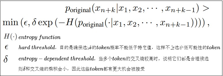
于是，Medusa從截斷采樣（Truncation Sampling）工作中汲取靈感，旨在擴大選擇原始模型可能接受的候選項。Medusa 根據原始模型的預測概率設定一個閾值，如果候選token超過了這個閾值，就會被接受該token 及其 prefix，并在這些token中做Greedy采樣選擇top-k。而這個閾值由原始模型的預測概率相關。

具體來說，作者采取hard threshold和entropy-dependent threshold的最小值來決定是否像在truncation sampling中那樣接受一個候選token。這確保了在解碼過程中選擇有意義的token和合理的延續。作者總是使用Greedy Decoding接受第一個token，確保每一步至少生成一個token。最后選擇被接受的解碼長度最長的候選序列作為最終結果。這種方法的好處是其適應性：如果你將采樣溫度設為零，它就簡單地回歸到最高效的形式Greedy Search。當你提高溫度時，此方法變得更加高效，允許更長的接受序列。

當概率分布中有個別token的概率很高，這時熵小， exp?(???(?)) 大，token接受的條件更嚴格。
當概率分布中每個token的概率比較平均時，熵大， exp?(???(?)) 小，token接受的條件寬松一些。

具體實現位于evaluate_posterior()函數中，這里不再贅述。

0x04 訓練

MEDUSA的這些分類頭需要經過訓練才能有比較好的預測效果。針對不同的條件，可以選擇不同的訓練方式：

MEDUSA-1：凍結原模型的backbone（包括原模型的解碼頭），只訓練增加的解碼頭。這種方案適用于計算資源比較少，或者不想影響原模型的效果的情況。還可以使用QLoRA對解碼頭進行訓練，進一步節省內存和計算資源。
MEDUSA-2：原模型和MEDUSA的解碼頭一起訓練。MEDUSA-1這樣的訓練方法雖然可以節省資源，但是并不能最大程度發揮多個解碼頭的加速效果，而MEDUSA-2則可以進一步發揮MEDUSA解碼頭的提速能力。而且，由于是基干模型與Medusa Heads一起進行訓練，確保了MEDUSA heads的分布與原始模型的分布保持一致，從而減輕了分布漂移問題，顯著提高Heads的準確性。MEDUSA-2適用于計算資源充足，或者從Base模型進行SFT的場景。

另外，如果原模型的SFT數據集是available的，那可以直接進行訓練。如果不能獲得原模型的SFT數據，或者原模型是經過RLHF訓練的，則可以通過self-distillation來獲取MEDUSA head的訓練數據。

4.1 MEDUSA-1

MEDUSA-1凍結了原模型的參數，而只對新增的解碼頭進行訓練。使用Medusa-1訓練Heads，主要計算Medusa Heads預測的結果與Ground Truth之間的交叉熵損失。具體計算為，給定位置 t+k+1 處的Ground Truth $y_{t+k+1}$ ,則第 k 個Head的訓練loss可以寫作：

\[\mathcal{L}_k=-\log p_t^{(k)}(y_{t+k+1}) \]

并且當k 較大時， $\mathcal{L}_k$ 也會隨之變大，因為當 k 變大時，靠后的Head的預測將更加不確定。為了平衡各個 Head 上 loss 的大小，因此在 $\mathcal{L}_k$ 上增加指數衰減的權重參數 $\lambda_k$ 來平衡不同head的損失。最終Medusa的損失計算如下：

\[\mathcal{L}_{\text{MEDUSA-l}}=\sum_{k=1}^K-\lambda_k\log p_t^{(k)}(y_{t+k+1}) \]

這里的 $\lambda_{k}$ 是每個解碼頭的縮放系數，是一系列超參。因為 k 越大，對應解碼頭的預測難度越大，loss也就越大，為了防止靠后的解碼頭過分主導訓練，因此使用一個縮放系數進行調整。實際使用中，$\lambda_{k}=0.8^{k}$。

4.2 MEDUSA-2

為了進一步提高Medusa Heads的準確性，MEDUSA-2把原模型和多個解碼頭一起訓練，因此各個解碼頭的準確率能達到更高的水平，acceleration rate也更高。但是為了保持原模型的輸出質量，需要一些特殊的訓練技巧。Medusa-2使用以下三個策略來實現這個目標。

Combined loss

為了保持backbone模型 next token預測的能力，需要將backbone模型的交叉熵損失 $L_{LM}$添加到Medusa損失中，即把原模型解碼頭的loss也加上。同時還需要添加一個權重因子 $\lambda_0$ 來平衡backbone和Medusa Heads之間的損失。具體如下式

\[\mathcal{L}_{\text{MEDUSA-}2}=\mathcal{L}_{\text{LM}}+\lambda_0\mathcal{L}_{\text{MEDUSA-}1} \\\mathcal{L}_{\text{LM}}=-\log p_t^{(0)}(y_{t+1}) \]

實際使用中，直接訓練時 $\lambda_0=0.2$，使用self-distillation時$\lambda_0=0.01$。

Differential learning rates

原模型已經是訓練好了的，，而 MEDUSA heads需要更多訓練，因此原模型和新加入的解碼頭使用相同的學習率并不合適。我們可以讓新的解碼頭使用更大的學習率，而原模型參數使用相對小的學習率，以實現 MEDUSA heads更快的收斂，同時保留backbone模型的能力。實踐中把學習率差距設為4倍，比如分別使用2e-3和5e-4。

Heads warmup

新加入的解碼頭在一開始訓練會有比較大的loss，從而導致更大的梯度，有可能損害原模型的能力。針對這個問題，可以使用兩階段訓練過程g的方式。在第一階段，先在MEDUSA-1的策略下僅訓練解碼頭，在第二階段，再進行MEDUSA-2的訓練。這其實相當于把 $\lambda_0$ 在訓練過程中逐漸增大。

4.3 代碼

我們再來看看一個已經訓練好的LLM如何適配MEDUSA，具體分為如下幾步：

添加解碼頭：在 LLM 最后一個隱藏層后添加若干個 MEDUSA 解碼頭。
初始化解碼頭：可使用隨機初始化，也可使用原始模型解碼頭的參數進行初始化，這樣可以加快訓練速度。
選擇訓練策略：根據實際情況選擇 MEDUSA-1 或 MEDUSA-2 策略。
準備訓練數據：可以復用原始模型的訓練數據，也可以使用自蒸餾方法生成訓練數據。
訓練：根據選擇的策略和數據，訓練 MEDUSA 解碼頭或同時微調 LLM。

訓練具體代碼如下。首先需要訓練幾個新增的頭，不同的頭預測的label的偏移量不同，所以可以組裝每個頭的topk作為候選。

# Customized for training Medusa heads
class CustomizedTrainer(Trainer):
    def compute_loss(self, model, inputs, return_outputs=False):
        """
        Compute the training loss for the model.

        Args:
            model (torch.nn.Module): The model for which to compute the loss.
            inputs (dict): The input data, including input IDs, attention mask, and labels.
            return_outputs (bool): Whether to return model outputs along with the loss.

        Returns:
            Union[float, Tuple[float, torch.Tensor]]: The computed loss, optionally with model outputs.
        """
        # DDP will give us model.module
        if hasattr(model, "module"):
            medusa = model.module.medusa
        else:
            medusa = model.medusa

        logits = model(
            input_ids=inputs["input_ids"], attention_mask=inputs["attention_mask"]
        )
        labels = inputs["labels"]
        # Shift so that tokens < n predict n
        loss = 0
        loss_fct = CrossEntropyLoss()
        log = {}
        for i in range(medusa):
            medusa_logits = logits[i, :, : -(2 + i)].contiguous()
            # 常規的標簽需要偏移1個位置, 由于不訓練LM Head，所以偏移2個位置.
            medusa_labels = labels[..., 2 + i :].contiguous()
            medusa_logits = medusa_logits.view(-1, logits.shape[-1])
            medusa_labels = medusa_labels.view(-1)
            medusa_labels = medusa_labels.to(medusa_logits.device)
            loss_i = loss_fct(medusa_logits, medusa_labels)
            loss += loss_i
            not_ignore = medusa_labels.ne(IGNORE_TOKEN_ID)
            medusa_labels = medusa_labels[not_ignore]

            # Add top-k accuracy
            for k in range(1, 2):
                _, topk = medusa_logits.topk(k, dim=-1)
                topk = topk[not_ignore]
                correct = topk.eq(medusa_labels.unsqueeze(-1)).any(-1)

        return (loss, logits) if return_outputs else loss

0x05 Decoding

5.1 示例

官方github源碼給出了前向傳播代碼如下。

@contextmanager
def timed(wall_times, key):
    start = time.time()
    torch.cuda.synchronize()
    yield
    torch.cuda.synchronize()
    end = time.time()
    elapsed_time = end - start
    wall_times[key].append(elapsed_time)

def medusa_forward(input_ids, model, tokenizer, medusa_choices, temperature, posterior_threshold, posterior_alpha, max_steps = 512):
    wall_times = {'medusa': [], 'tree': [], 'posterior': [], 'update': [], 'init': []}
    
    with timed(wall_times, 'init'):
        if hasattr(model, "medusa_choices") and model.medusa_choices == medusa_choices:
            # Load the cached medusa buffer
            medusa_buffers = model.medusa_buffers
        else:
            # Initialize the medusa buffer
            medusa_buffers = generate_medusa_buffers(
                medusa_choices, device=model.base_model.device
            )
        model.medusa_buffers = medusa_buffers
        model.medusa_choices = medusa_choices

        # Initialize the past key and value states
        if hasattr(model, "past_key_values"):
            past_key_values = model.past_key_values
            past_key_values_data = model.past_key_values_data
            current_length_data = model.current_length_data
            # Reset the past key and value states
            current_length_data.zero_()
        else:
            (
                past_key_values,
                past_key_values_data,
                current_length_data,
            ) = initialize_past_key_values(model.base_model)
            model.past_key_values = past_key_values
            model.past_key_values_data = past_key_values_data
            model.current_length_data = current_length_data

        input_len = input_ids.shape[1]
        reset_medusa_mode(model)
        medusa_logits, logits = initialize_medusa(
                input_ids, model, medusa_buffers["medusa_attn_mask"], past_key_values
        )
    new_token = 0

    for idx in range(max_steps): 
        with timed(wall_times, 'medusa'):
            candidates, tree_candidates = generate_candidates(
                    medusa_logits,
                    logits,
                    medusa_buffers["tree_indices"],
                    medusa_buffers["retrieve_indices"],
                )

        with timed(wall_times, 'tree'):
            medusa_logits, logits, outputs = tree_decoding(
                    model,
                    tree_candidates,
                    past_key_values,
                    medusa_buffers["medusa_position_ids"],
                    input_ids,
                    medusa_buffers["retrieve_indices"],
                )

        with timed(wall_times, 'posterior'):
            best_candidate, accept_length = evaluate_posterior(
                    logits, candidates, temperature, posterior_threshold, posterior_alpha
                )
        
        with timed(wall_times, 'update'):
            input_ids, logits, medusa_logits, new_token = update_inference_inputs(
                    input_ids,
                    candidates,
                    best_candidate,
                    accept_length,
                    medusa_buffers["retrieve_indices"],
                    outputs,
                    logits,
                    medusa_logits,
                    new_token,
                    past_key_values_data,
                    current_length_data,
                )

        if tokenizer.eos_token_id in input_ids[0, input_len:].tolist():
            break

    return input_ids, new_token, idx, wall_times

調用方法樣例如下。

import os
os.environ["CUDA_VISIBLE_DEVICES"] = "3" # define GPU id, remove if you want to use all GPUs available
import torch
from tqdm import tqdm
import time
from contextlib import contextmanager
import numpy as np
from medusa.model.modeling_llama_kv import LlamaForCausalLM as KVLlamaForCausalLM
from medusa.model.medusa_model import MedusaModel
from medusa.model.kv_cache import *
from medusa.model.utils import *
from medusa.model.medusa_choices import *
import transformers
from huggingface_hub import hf_hub_download

# 加載模型
model_name = 'FasterDecoding/medusa-vicuna-7b-v1.3'
model = MedusaModel.from_pretrained(
    model_name,
    medusa_num_heads = 4,
    torch_dtype=torch.float16,
    low_cpu_mem_usage=True,
    device_map="auto"
)
tokenizer = model.get_tokenizer()

medusa_choices = mc_sim_7b_63

# 設置推理參數
temperature = 0.
posterior_threshold = 0.09
posterior_alpha = 0.3

# 設置prompt
prompt = "A chat between a curious user and an artificial intelligence assistant. The assistant gives helpful, detailed, and polite answers to the user's questions. USER: Hi, could you share a tale about a charming llama that grows Medusa-like hair and starts its own coffee shop? ASSISTANT:"

# 執行推理
with torch.inference_mode():
    input_ids = tokenizer([prompt]).input_ids
    output_ids, new_token, idx, wall_time = medusa_forward(
                    torch.as_tensor(input_ids).cuda(),
                    model,
                    tokenizer,
                    medusa_choices,
                    temperature,
                    posterior_threshold,
                    posterior_alpha,
                )
    output_ids = output_ids[0][len(input_ids[0]) :]
    print("Output length:", output_ids.size(-1))
    print("Compression ratio:", new_token / idx)
    
# 解碼
output = tokenizer.decode(
                    output_ids,
                    spaces_between_special_tokens=False,
                )
print(output)

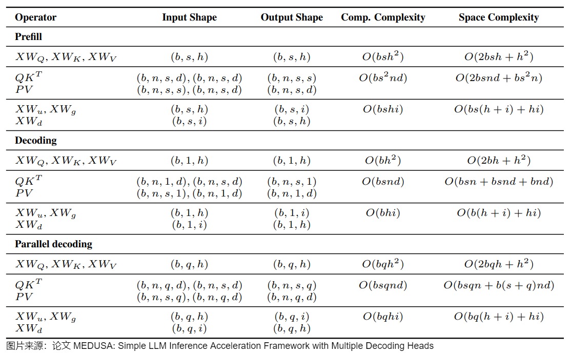
5.2 計算和空間復雜度

下圖給出了prefill，decoding、MEDUSA decoding階段的計算和空間復雜度。

b是batch size。
s是序列長度。
h是hidden dimension。
i是intermediate dimension。
n是注意力頭個數。
d是頭維度。
q是MEDUSA的候選長度。

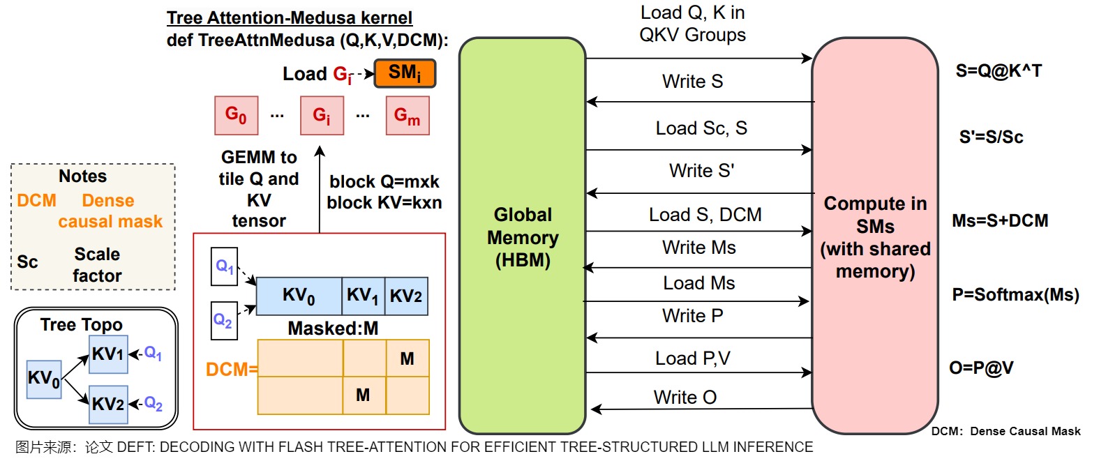
另外，下圖給出了Medusa 的操作流程。當沒有算子融合或者Tiling策略時，$QK^?$，DCM(Dense Causal Mask)，Softmax都會導致顯存和片上緩存之間大量的IO操作。

0xFF 參考

SpecInfer: Accelerating Generative Large Language Model Serving with Speculative Inference and Token Tree Verification

Medusa: Simple LLM Inference Acceleration Framework with Multiple Decoding Heads

LLM 投機解碼 & 美杜莎(Medusa)實現 AI閑談

【手撕LLM-Medusa】并行解碼范式: 美杜莎駕到, 通通閃開！！小冬瓜AIGC

方佳瑞：大模型推理妙招—投機采樣（Speculative Decoding）

[Transformer 101系列] 深入LLM投機采樣(上) aaronxic

https://github.com/FasterDecoding/Medusa/blob/main/notebooks/medusa_introduction.ipynb

Medusa: Simple LLM Inference Acceleration Framework with Multiple Decoding Heads, Jan 2024, Princeton University. Proceedings of the ICML 2024.

[2401.10774] Medusa: Simple LLM Inference Acceleration Framework with Multiple Decoding Heads

Medusa: Simple LLM Inference Acceleration Framework with Multiple Decoding Heads

GitHub - FasterDecoding/Medusa: Medusa: Simple Framework for Accelerating LLM Generation with Multiple Decoding Heads

LLM推理加速之Medusa：Blockwise Parallel Decoding的繼承與發展方佳瑞

方佳瑞：LLM推理加速的文藝復興：Noam Shazeer和Blockwise Parallel Decoding?

萬字綜述 10+ 種 LLM 投機采樣推理加速方案 AI閑談

[2401.07851] Unlocking Efficiency in Large Language Model Inference: A Comprehensive Survey of Speculative Decoding

速覽Medusa與Lookahead投機推理是阿沅啊

開源進展 | Medusa: 使用多頭解碼，將大模型推理速度提升2倍以上洪洗象

arXiv:1811.03115: Berkey, Google Brain, Blockwise Parallel Decoding for Deep Autoregressive Models.

arXiv:2211.17192: Google Research, Fast Inference from Transformers via Speculative Decoding

arXiv:2202.00666: ETH Zu?rich、University of Cambridge，Locally Typical Sampling

[4] arXiv:2106.05234: Dalian University of Technology、Princeton University、Peking University、Microsoft Research Asia，Do Transformers Really Perform Bad for Graph Representation?

3萬字詳細解析清華大學最新綜述工作：大模型高效推理綜述 zenRRan

大模型推理加速-MEDUSA Linsight

LLM推理加速-Medusa uuuuu

【手撕LLM-Medusa】并行解碼范式: 美杜莎駕到, 通通閃開！！小冬瓜AIGC

Blockwise Parallel Decoding 論文解讀 AI閑談

LLM 投機解碼 & 美杜莎(Medusa)實現 AI閑談

https://sites.google.com/view/medusa-llm

https://github.com/FasterDecoding/Medusa

百川 Clover：優于 Medusa 的投機采樣 AI閑談

[2405.00263] Clover: Regressive Lightweight Speculative Decoding with Sequential Knowledge

Hydra: Sequentially-Dependent Draft Heads for Medusa Decoding 灰瞳六分儀

Hydra: Sequentially-Dependent Draft Heads for Medusa Decoding