scipy 用于以下的科學(xué)領(lǐng)域中的Subpackage及簡(jiǎn)述

• cluster：用于聚類算法
• constants： 用于物理里面的常數(shù)，例如光速c
• integrate: 積分和微分方程
• interpolate：插值
• signal：信號(hào)處理
• linalg：線性代數(shù)
• ndimage：N緯圖形
• optimize：最優(yōu)化
• sparse：稀疏矩陣
• stats：統(tǒng)計(jì)分布

常數(shù)和特殊函數(shù)實(shí)例

from scipy import constants as C
print(C.c) # 真空中的光速
print(C.c) # 普朗克常量
#299792458.0
#6.62607015e-34

# 1英里等于多少米, 1英寸等于多少米, 1克等于多少千克, 1磅等于多少千克
print(C.mile)
print(C.inch)
print(C.gram)
print(C.pound)

1609.3439999999998
0.0254
0.001
0.45359236999999997

• $log1p$函數(shù)：做平滑處理，在有時(shí)能使數(shù)據(jù)更接近與高斯分布
  $log1p(x)=log(x+1)$ 即$ln(x+1)$
  因此當(dāng)數(shù)據(jù)很小的時(shí)候，$ln(x+1)=x$ 等價(jià)無窮小
  $expm1(x)=exp(x)?1$

import numpy as np
import scipy.special as S
print(1 + 1e-20)# 1+10的負(fù)20次方
print(np.log(1+1e-20))
print(S.log1p(1e-20))

1.0
0.0
1e-20

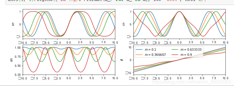
m = np.linspace(0.1, 0.9, 4)
u = np.linspace(-10, 10, 200)
results = S.ellipj(u[:, None], m[None, :])
print([y.shape for y in results])

#%figonly=使用廣播計(jì)算得到的`ellipj()`返回值
import matplotlib.pyplot as plt
fig, axes = pl.subplots(2, 2, figsize=(12, 4))1
labels = ["$sn$", "$cn$", "$dn$", "$\phi$"]
for ax, y, label in zip(axes.ravel(), results, labels):
    ax.plot(u, y)
    ax.set_ylabel(label)
    ax.margins(0, 0.1)
    
axes[1, 1].legend(["$m={:g}$".format(m_) for m_ in m], loc="best", ncol=2)

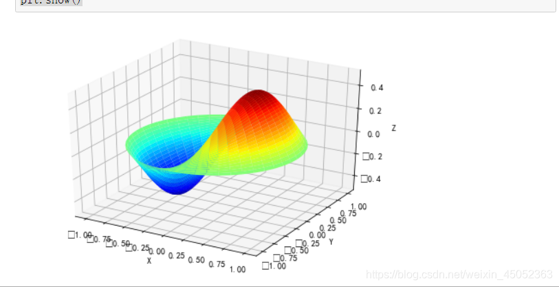
• 貝塞爾函數(shù)是貝塞爾具有實(shí)階或復(fù)階alpha的微分方程的一系列解決方案：
  $$x^2\frac{d^{2}y}{d{x}^2}+x\frac{dy}{dx}+(x^2?a^2)y=0$$
  在其他用途??中，這些功能會(huì)出現(xiàn)在波傳播問題中，例如薄磁鼓鼓頭的振動(dòng)模式。
  這是一個(gè)固定在邊緣的圓形鼓頭示例：

from scipy import special
def drumhead_height(n, k, distance, angle, t):
    kth_zero = special.jn_zeros(n, k)[-1]
    return np.cos(t) * np.cos(n*angle) * special.jn(n, distance*kth_zero)
theta = np.r_[0:2*np.pi:50j]
radius = np.r_[0:1:50j]
x = np.array([r * np.cos(theta) for r in radius])
y = np.array([r * np.sin(theta) for r in radius])
z = np.array([drumhead_height(1, 1, r, theta, 0.5) for r in radius])

import matplotlib.pyplot as plt
from mpl_toolkits.mplot3d import Axes3D
from matplotlib import cm
fig = plt.figure()
ax = Axes3D(fig)
ax.plot_surface(x, y, z, rstride=1, cstride=1, cmap=cm.jet)
ax.set_xlabel('X')
ax.set_ylabel('Y')
ax.set_zlabel('Z')
plt.show()