TensorFlow2學習(1)
Tensorflow2學習(1)1 TensorFlow2學習1.1 張量(Tensor)1.1.1張量是多維數組(列表),用階表示張量的維數:1.1.2創建一個Tensor1.2 常用函數1.3 簡單實踐(鳶尾花數據讀取與神經網絡分類)1.3.1 鳶尾花數據讀取1.3.2 神經網絡分類
1 TensorFlow2學習
1.1 張量(Tensor)
1.1.1張量是多維數組(列表),用階表示張量的維數:
| 維數 | 階 | 名稱 | 例子 |
|---|---|---|---|
| 0-D | 0 | scalar 標量 | s=1 2 3 |
| 1-D | 1 | vector 向量 | s=[1,2,3] |
| 2-D | 2 | matrix 矩陣 | s=[[1,2,3],[1,2,3],[1,2,3]] |
| n-D | 3 | tensor 張量 | s=[[[ ]]] 其中左側中括號有n個 |
1.1.2創建一個Tensor
1)tf.constant(張量內容,dtype=數據類型(可選))
import tensorflow as tf
import os
os.environ["TF_CPP_MIN_LOG_LEVEL"] = "2"
?
a = tf.constant([1, 5],dtype=tf.int64)
print(a)
print(a.dtype)
print(a.shape)
?
#結果顯示
tf.Tensor([1 5], shape=(2,), dtype=int64)
<dtype: 'int64'>
(2,)
注:張量的形狀看shape的逗號隔開了幾個數字,隔開了幾個數字,張量就是幾維。
2)tf.convert_to_tensor(數據名,dtype=數據類型(可選)) 將numpy的數據類型轉換為tensor數據類型。
import tensorflow as tf
import numpy as np
import os
os.environ["TF_CPP_MIN_LOG_LEVEL"] = "2"
?
a = np.arange(0, 5)
b = tf.convert_to_tensor(a, dtype=tf.int64)
print(a)
print(b)
?
#結果顯示
[0 1 2 3 4]
tf.Tensor([0 1 2 3 4], shape=(5,), dtype=int64)
3)tf.fill(維度,指定值) 創建全為指定值的張量,其中指定值只能為標量。
a = tf.fill([2, 3], 9)
print(a)
?
#結果顯示
tf.Tensor(
[[9 9 9]
 [9 9 9]], shape=(2, 3), dtype=int32)
4)tf.random.normal(維度,mean=均值,stddev=標準差) 生成正態分布的隨機數,默認均值為0,標準差為1
tf.random.truncated_normal(維度,mean=均值,stddev=標準差) 生成截斷式正態分布的隨機數,生成的數更向均值集中。
a = tf.random.normal([2, 2], mean=0.3, stddev=2)
b = tf.random.truncated_normal([2, 2], mean=0.3, stddev=2)
print(a)
print(b)
?
#結果顯示
tf.Tensor(
[[-0.41351897  1.8662729 ]
 [ 2.200518    1.3296602 ]], shape=(2, 2), dtype=float32)
tf.Tensor(
[[ 1.5761657  1.201687 ]
 [ 1.9042709 -0.7466951]], shape=(2, 2), dtype=float32)
4)tf.random.uniform(維度,minval=最小值,maxval=最大值) 生成均勻分布的隨機數,生成數區間是前開后閉區間。
a = tf.random.uniform([2, 2], minval=-2, maxval=2)
print(a)
?
#結果顯示
tf.Tensor(
[[ 0.2742386  -0.69904184]
 [ 1.3488121  -0.7883253 ]], shape=(2, 2), dtype=float32)
1.2 常用函數
1)tf.cast(張量名,dtype=數據類型) 強制tensor轉換為該數據類型
2)tf.reduce_min(張量名) 計算張量維度上元素的最小值
3)tf.reduce_max(張量名) 計算張量維度上元素的最大值
x1 = tf.constant([1, 2, 3], dtype=tf.int64)
print(x1)
x2 = tf.cast(x1, tf.float32)
print(x2)
x3 = tf.reduce_min(x1)
x4 = tf.reduce_max(x2)
print(x3, x4)
?
#結果顯示
tf.Tensor([1 2 3], shape=(3,), dtype=int64)
tf.Tensor([1. 2. 3.], shape=(3,), dtype=float32)
tf.Tensor(1, shape=(), dtype=int64) tf.Tensor(3.0, shape=(), dtype=float32)
4)tf.reduce_mean(張量名,axis=操作軸) 計算張量沿著指定維度的平均值,其中axis為1,表示行,為0表示列,若axis沒寫,則對整個張量求平均,先列求,再行求。
5)tf.reduce_sum(張量名,axis=操作軸) 計算張量沿著指定維度的和。
x = tf.constant([[1, 2, 3], [3, 2, 3]], dtype=tf.float32)
print(x)
print(tf.reduce_mean(x), tf.reduce_sum(x, axis=1))
?
#結果顯示
tf.Tensor(
[[1. 2. 3.]
 [3. 2. 3.]], shape=(2, 3), dtype=float32)
tf.Tensor(2.3333333, shape=(), dtype=float32) tf.Tensor([6. 8.], shape=(2,), dtype=float32)
6)tf.Variable(初始值) 將變量標記為“可訓練”,被標記的變量會在反向傳播中記錄梯度信息。神經網絡訓練中,常用該函數標記待訓練參數。
w = tf.Variable(tf.random.uniform([2, 2], minval=0, maxval=1))
print(x)
?
#結果顯示
<tf.Variable 'Variable:0' shape=(2, 2) dtype=float32, numpy=
array([[0.7305305 , 0.7579589 ],
       [0.02064288, 0.32717478]], dtype=float32)>
注:可以用來表示損失函數loss的參數w,即將w標記為可訓練變量。
7)tensorflow中的數學運算
-
四則運算:tf.add;tf.subtract;tf.multiply;tf.divide。這些四則運算張量維度必須一樣
-
平方、次方與開方:tf.square;tf.pow;tf.sqrt
-
矩陣乘:tf.matmul
8)tf.data.Dataset.from_tensor_slices((輸入特征,標簽)) 切分傳入張量的第一維度,生成輸入特征/標簽對,構建數據集。該方法可以讀取numpy與tensor兩種格式的數據。
feature = tf.constant([1, 3, 10, 24])
labels = tf.constant([0, 0, 1, 1])
dataset = tf.data.Dataset.from_tensor_slices((feature, labels))
print(dataset)
for i in dataset:
    print(i)
?
#結果顯示
<TensorSliceDataset shapes: ((), ()), types: (tf.int32, tf.int32)>
(<tf.Tensor: id=9, shape=(), dtype=int32, numpy=1>, <tf.Tensor: id=10, shape=(), dtype=int32, numpy=0>)
(<tf.Tensor: id=11, shape=(), dtype=int32, numpy=3>, <tf.Tensor: id=12, shape=(), dtype=int32, numpy=0>)
(<tf.Tensor: id=13, shape=(), dtype=int32, numpy=10>, <tf.Tensor: id=14, shape=(), dtype=int32, numpy=1>)
(<tf.Tensor: id=15, shape=(), dtype=int32, numpy=24>, <tf.Tensor: id=16, shape=(), dtype=int32, numpy=1>)
9)tf.GradientTape() 用它的with結構記錄計算過程,gradient求出張量的梯度,即求導。
其結構一般為:
with tf.GradientTape() as tape:
    若干個計算過程
grad = tape.gradient(函數, 對誰求導)
下面舉個例子:其中損失函數為w的平方,w=3.0
with tf.GradientTape() as tape:
    w = tf.Variable(3.0)
    loss = tf.pow(w, 2)
grad = tape.gradient(loss, w)
print(grad)
?
#結果顯示
tf.Tensor(6.0, shape=(), dtype=float32)
10)enumerate(列表名) 是python的內建函數,它可以遍歷每個元素(如列表、元組或字符串),組合形式為:索引+元素,常在for循環中使用。
seq = ['one', 'two', 'three']
for i, element in enumerate(seq):
    print(i, element)
?
#結果顯示
0 one
1 two
2 three
11)tf.one_hot(待轉換數據,depth=幾分類) 在分類問題中,用獨熱碼,即one_hot做標簽,‘1’表示是,‘0’表示非,將待轉換數據,轉換為one_hot形式的數據進行輸出。
classes = 5
labels = tf.constant([1, 2, 3])
output = tf.one_hot(labels, classes)
print(output)
?
#結果顯示
tf.Tensor(
[[0. 1. 0. 0. 0.]
 [0. 0. 1. 0. 0.]
 [0. 0. 0. 1. 0.]], shape=(3, 5), dtype=float32)
12)tf.nn.softmax(待轉換數據) 使n個輸出變成0~1的值,且其和為1。
y = tf.Variable([1.02, 2.30, -0.19])
y_pro = tf.nn.softmax(y)
print("After softmax, y_pro is:", y_pro)
?
#結果顯示
After softmax, y_pro is: tf.Tensor([0.2042969  0.73478234 0.06092078], shape=(3,), dtype=float32)
13)assign_sub(w要自減的內容) 賦值操作,更新參數的值并返回。要更新的參數的前提是,其是可訓練的,即初始w值是variable構建的。
w = tf.Variable(3)
w.assign_sub(1) # 實現w-1功能,即自減
print(w)
?
#結果顯示
<tf.Variable 'Variable:0' shape=() dtype=int32, numpy=2>
14)tf.argmax(張量名,axis=操作軸) 返回張量沿指定維度最大值的索引。
x = np.array([[1, 2, 3], [2, 3, 4], [4, 5, 6]])
print(x)
print(tf.argmax(x, axis=1))
print(tf.argmin(x, axis=0))
?
#結果顯示
[[1 2 3]
 [2 3 4]
 [4 5 6]]
tf.Tensor([2 2 2], shape=(3,), dtype=int64)
tf.Tensor([0 0 0], shape=(3,), dtype=int64)
1.3 簡單實踐(鳶尾花數據讀取與神經網絡分類)
1.3.1 鳶尾花數據讀取
from sklearn import datasets
from pandas import DataFrame
import pandas as pd
?
x_data = datasets.load_iris().data
y_data = datasets.load_iris().target
#print('鳶尾花數據:\n', x_data)
#print('鳶尾花標簽:\n', y_data)
?
x_data = DataFrame(x_data, columns=['花萼長度', '花萼寬度', '花瓣長度', '花瓣寬度'])# 將其變成表格形式,并為每一列增加中文標簽
pd.set_option('display.unicode.east_asian_width', True)# 設置表格為列名對其
print('鳶尾花數據:\n', x_data)
?
x_data['類別'] = y_data # 為x_data增加一列類別,即原來定義的y_data
print('增加一列后的表格為:\n', x_data)
?
#結果顯示
鳶尾花數據:
      花萼長度  花萼寬度  花瓣長度  花瓣寬度
0         5.1       3.5       1.4       0.2
..        ...       ...       ...       ...
149       5.9       3.0       5.1       1.8
?
[150 rows x 4 columns]
增加一列后的表格為:
      花萼長度  花萼寬度  花瓣長度  花瓣寬度  類別
0         5.1       3.5       1.4       0.2     0
..        ...       ...       ...       ...   ...
149       5.9       3.0       5.1       1.8     2
?
[150 rows x 5 columns]
1.3.2 神經網絡分類
實現該功能我們可以分三步走:
-
準備數據
-
數據集讀入
-
數據集亂序
-
生成訓練集和測試集(即x_train/y_train,x_test/y_test)
-
配成(輸入特征,標簽)對,每次讀入一小撮(batch)
-
搭建網絡
-
定義神經網絡中所有可訓練參數
-
參數優化
-
嵌套循環迭代,with結構更新參數,顯示當前loss
-
注:還可以進行以下操作
1)測試結果
-
計算當前參數前向傳播后的準確率,顯示當前acc
2)acc/loss可視化
以下為一個神經網絡實現鳶尾花分類示例:
import tensorflow as tf
from sklearn import datasets
import matplotlib.pyplot as plt
import numpy as np
?
# 第一步-準備數據-數據讀取
x_data = datasets.load_iris().data
y_data = datasets.load_iris().target
?
# 第一步-準備數據-打亂數據
np.random.seed(1) # 使用相同的seed打亂,保證輸入的數據與標簽一一對應
np.random.shuffle(x_data) # 生成隨機列表
np.random.seed(1)
np.random.shuffle(y_data)
tf.random.set_seed(1)
?
# 第一步-準備數據-分成訓練集和測試集
x_train = x_data[:-30] # 由開頭到倒數第30個
y_train = y_data[:-30]
x_test = x_data[-30:] # 由倒數第30個到最后
y_test = y_data[-30:]
?
# 為防止數據集出現計算上的錯誤,我們將數據集轉換類型
x_train = tf.cast(x_train, dtype=tf.float32)
x_test = tf.cast(x_test, dtype=tf.float32)
?
# 第一步-準備數據-特征值與標簽配對,并以batch形式輸入
train_fl = tf.data.Dataset.from_tensor_slices((x_train, y_train)).batch(32)
test_fl = tf.data.Dataset.from_tensor_slices((x_test, y_test)).batch(32)
?
# 第二步-搭建網絡-定義所有相關參數(這一步可以在訓練等模型寫完后再完成)
w1 = tf.Variable(tf.random.truncated_normal([4, 3], stddev=0.1))
b1 = tf.Variable(tf.random.truncated_normal([3], stddev=0.1))
lr = 0.1 # 學習率為0.1
train_loss_result = [] # 每輪的loss記錄于此,為后面的loss圖像提供數據
test_acc = [] # 每輪的準確率記錄于此,為后面的acc圖像提供數據
epoch = 500 # 循環次數
loss_all = 0 # 每輪分4個step,loss_all記錄四個step生成的4個loss的和
?
# 第三步-參數優化-訓練模型部分
for epoch in range(epoch): # 數據集級別的循環,每個epoch循環一次數據集
for step, (x_train, y_train) in enumerate(train_fl): # batch級別的循環,每個step循環一次batch
with tf.GradientTape() as tape:
y = tf.matmul(x_train, w1) + b1 # 全連接層
y = tf.nn.softmax(y) # 輸出0~1的真實值
y_ = tf.one_hot(y_train, depth=3) # 預測值
loss = tf.reduce_mean(tf.square(y_ - y)) # 損失函數
loss_all += loss.numpy() # 將每個step計算出的loss累加,為后面求loss平均值提供數據
grads = tape.gradient(loss, [w1, b1])
# 實現w與b的梯度更新:w1=w1-lr*w1_grad ,b1同理
w1.assign_sub(lr * grads[0])
b1.assign_sub(lr * grads[1])
print('Epoch {}, loss: {}'.format(epoch, loss_all/4))
train_loss_result.append(loss_all / 4) # 將4個step的loss求平均記錄在變量中
loss_all = 0 # 將loss_all歸零,為記錄下一個epoch做準備
?
# 第四步-預測模型部分
total_correct, total_number = 0, 0 # 前者為測試結果為正確的數量,后者為樣本總數量,都初始化為0
for x_test, y_test in test_fl: # 因為我們每個step為32,而我們數據只有30個,所以這里不使用enumerate
y = tf.matmul(x_test, w1) + b1
y = tf.nn.softmax(y)
pred = tf.argmax(y, axis=1) # 返回預測值中最大的索引,即預測的分類
pred = tf.cast(pred, dtype=y_test.dtype)
correct = tf.cast(tf.equal(pred, y_test), dtype=tf.int32) # 預測正確的結果保留下來
correct = tf.reduce_sum(correct)
total_correct += int(correct)
total_number += x_test.shape[0]
acc = total_correct / total_number
test_acc.append(acc)
print('Test_acc:', acc)
print('---------------------------')
?
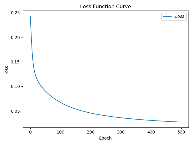
# 第五步-acc/loss可視化
plt.title('Loss Function Curve')
plt.xlabel('Epoch')
plt.ylabel('loss')
# plt.rcParams['font.sans-serif'] = ['FangSong']
# plt.rcParams['axes.Unicode_minus'] = False
plt.plot(train_loss_result, label='$Loss$')
plt.legend()
plt.show()
?
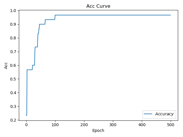
plt.title('Acc Curve')
plt.xlabel('Epoch')
plt.ylabel('Acc')
plt.plot(test_acc, label='$Accuracy$')
plt.legend()
plt.show()
?
#結果顯示
---------------------------
Epoch 499, loss: 0.02722732489928603
Test_acc: 0.9666666666666667
---------------------------

 浙公網安備 33010602011771號