吹靜靜

歡迎QQ交流：592590682

ClickHouse在做SQL查詢時要盡量遵循的原則

1.大表在左，小表在右，否則會造成右表加載數據量太大，大量消耗內存資源；

2.如果join的右表為大表，則需要將右表寫成子查詢，在子查詢中將右表的條件都加上，并進行列裁剪，這樣可以有效減少數據加載；

3.where條件中只放左表的條件，如果放右表的條件將在下推階段右表條件不會生效，將右表條件放到join的子查詢中去。

select ...
from t_all
join ( -- 右表本身直接走本地表
  select ...
  from t_local
  where t_local.filter = xxx -- 盡可能手動將條件放在子查詢中
)
where
  t_local.f = xxx -- 當前版本不支持自動下推到JOIN查詢中，需要手動修改
  and t_all.f in (
    select ... from xxx -- 若能將子查詢作為篩選條件更佳
  )

ClickHouse執行計劃分析

此執行計劃分析是在多分片單副本的ClickHouse環境中執行的。

準備數據

-- 建表語句
CREATE TABLE dw_local.t_a on cluster cluster_name (
`aid` Int64,
`score` Int64,
`shard` String,
`_sign` Int8,
`_version` UInt64
) ENGINE = ReplicatedReplacingMergeTree('/clickhouse/table/{shard}/t_a', '{replica}')
ORDER BY (aid);
CREATE TABLE dw_dist.t_a on cluster cluster_name as dw_local.t_a ENGINE = Distributed('cluster_name', 'dw_local', 't_a', sipHash64(shard));
CREATE VIEW dw.t_a on cluster cluster_name as select * from dw_dist.t_a final where _sign = 1;

CREATE TABLE dw_local.t_b on cluster cluster_name (
`bid` Int64,
`aid` Int64,
`shard` String,
`_sign` Int8,
`_version` UInt64
) ENGINE = ReplicatedReplacingMergeTree('/clickhouse/table/{shard}/t_b', '{replica}')
ORDER BY (bid);
CREATE TABLE dw_dist.t_b on cluster cluster_name as dw_local.t_b ENGINE = Distributed('cluster_name', 'dw_local', 't_b', sipHash64(shard));
CREATE VIEW dw.t_b on cluster cluster_name as select * from dw_dist.t_b final where _sign = 1;


-- 插入數據
insert into dw_dist.t_a (aid, score, shard, _sign, _version) values(1, 1, 's1', 1, 1);
insert into dw_dist.t_a (aid, score, shard, _sign, _version) values(2, 1, 's2', 1, 2);
insert into dw_dist.t_b (bid, aid, shard, _sign, _version) values(1, 1, 's1', 1, 1);
insert into dw_dist.t_b (bid, aid, shard, _sign, _version) values(2, 2, 's2', 1, 2);
insert into dw_dist.t_b (bid, aid, shard, _sign, _version) values(3, 0, 's1', 1, 3);
insert into dw_dist.t_b (bid, aid, shard, _sign, _version) values(4, 1, 's2', 1, 4);

案例1

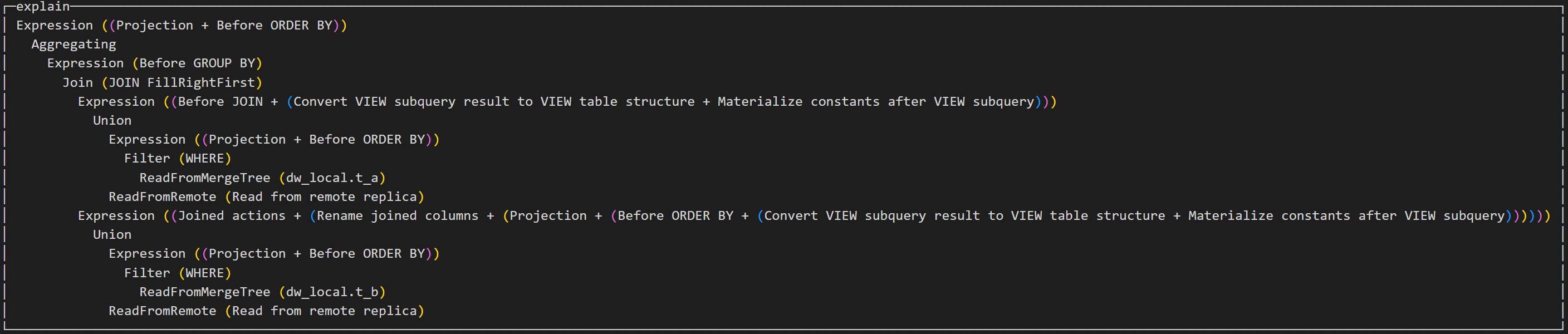
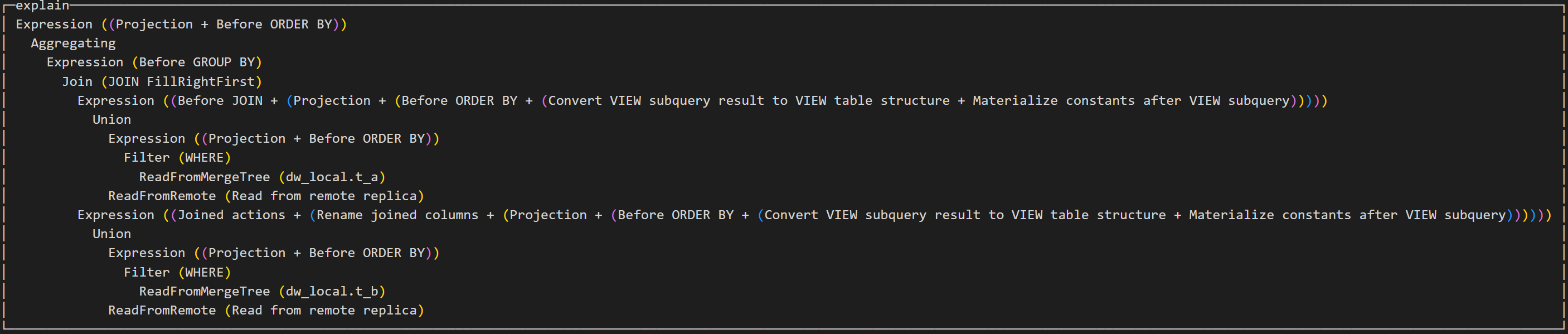
explain select a.aid as aid, b.bid as bid, count(*) as ct from dw.t_a as a join dw.t_b as b on a.aid = b.aid group by aid, bid;

通過執行計劃可以看到，左表和右表的執行計劃基本一樣，先將遠程節點上的表數據拉取到本地，然后和本地表的數據進行union操作，然后左表和右表進行join操作，最后進行group by操作。

案例2

explain select a.aid as aid, b.bid as bid, count(*) as ct from dw.t_b as b join dw.t_a as a on a.aid = b.aid group by aid, bid;

此SQL和案例1SQL相比只是將左右表的順序調換，此次表的執行順序只是調換了一下，從左到右執行。

案例3

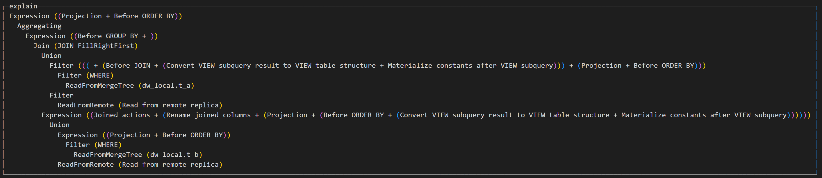
explain select a.aid as aid, b.bid as bid, count(*) as ct from dw.t_a as a join dw.t_b as b on a.aid = b.aid where a.aid=1 group by aid, bid;

此SQL和案例1SQL相比添加了左表的where條件，執行計劃中將條件放在了左表進行數據加載。

案例4

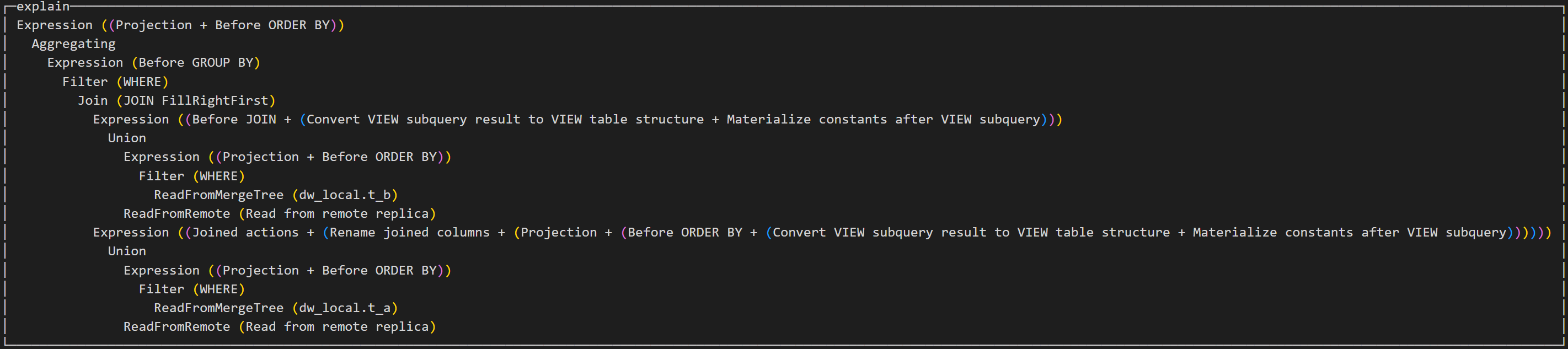
explain select a.aid as aid, b.bid as bid, count(*) as ct from dw.t_b as b join dw.t_a as a on a.aid = b.aid where a.aid=1 group by aid, bid;

此SQL中的左表表無過濾條件，右表存在過濾條件，執行計劃并不會將右表的條件放到拉取數據的階段。

案例5

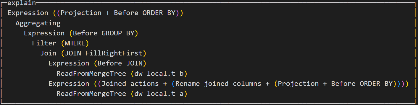
explain select a.aid as aid, b.bid as bid, count(*) as ct from dw_local.t_a as a join dw_local.t_b as b on a.aid = b.aid where a.aid=1 group by aid, bid;

如果所有表都采用本地表，而不是分布式表，則在數據加載階段不會拉取遠程節點的數據。

案例6

explain select a.aid as aid, b.bid as bid, count(*) as ct from dw_local.t_b as b join dw_local.t_a as a on a.aid = b.aid where a.aid=1 group by aid, bid;

調換左右表順序，同案例5結果相同。

案例7

explain select a.aid as aid, b.bid as bid, count(*) as ct from (
    select * from dw.t_a
) as a join dw.t_b as b on a.aid = b.aid group by aid, bid;

左表為子查詢時，左表也會走分布式表查詢方式拉取數據，有文章說左表為子查詢的情況下會導致左表走本地查詢策略，不走分布式查詢策略，可能是版本原因，我們測試過程中沒有出現類似情況。

參考文章：https://www.infoq.cn/article/blvraUL5LEImRzuWH56e

posted on 2023-02-03 14:08 吹靜靜閱讀(1274) 評論(0) 收藏舉報

刷新頁面返回頂部