
【自動微分實現(xiàn)】反向OO實現(xiàn)自動微分(Pytroch核心機制)
【自動微分實現(xiàn)】反向OO實現(xiàn)自動微分(Pytroch核心機制)
寫【自動微分】原理和實現(xiàn)系列文章,存粹是為了梳理在 MindSpore 當SE時候最核心的自動微分原理。網(wǎng)上看了很多文章,基本上都是很零散,當然Automatic Differentiation in Machine Learning: a Survey[1] 這篇文章是目前ZOMI覺得比較好關(guān)于自動微分的綜述論文。
- 【自動微分原理】01. 一文看懂AD原理
- 【自動微分原理】02. AD的正反向模式
- 【自動微分原理】03. AD常用實現(xiàn)方案
- 【自動微分原理】04. 正向OO實現(xiàn)自動微分
- 【自動微分原理】05. 反向OO實現(xiàn)自動微分(Pytroch核心機制)
這里記錄一下使用操作符重載(OO)編程方式的自動微分,其中數(shù)學實現(xiàn)模式則是使用反向模式(Reverse Mode),綜合起來就叫做反向OO實現(xiàn)AD啦。
基礎知識
下面一起來回顧一下操作符重載和反向模式的一些基本概念,然后一起去嘗試著用Python去實現(xiàn)Pytorch這個AI框架中最核心的自動微分機制是如何實現(xiàn)的。
操作符重載 OO
操作符重載:操作符重載或者稱運算重載(Operator Overloading,OO),利用現(xiàn)代語言的多態(tài)特性(例如C++/JAVA/Python等高級語言),使用操作符重載對語言中基本運算表達式的微分規(guī)則進行封裝。同樣,重載后的操作符在運行時會記錄所有的操作符和相應的組合關(guān)系,最后使用鏈式法則對上述基本表達式的微分結(jié)果進行組合完成自動微分。
在具有多態(tài)特性的現(xiàn)代編程語言中,運算符重載提供了實現(xiàn)自動微分的最直接方式,利用了編程語言的第一特性(first class feature),重新定義了微分基本操作語義的能力。
在 C++ 中使用運算符重載實現(xiàn)的流行工具是 ADOL-C(Walther 和 Griewank,2012)。 ADOL-C 要求對變量使用啟用 AD 的類型,并在 Tape 數(shù)據(jù)結(jié)構(gòu)中記錄變量的算術(shù)運算,隨后可以在反向模式 AD 計算期間“回放”。 Mxyzptlk 庫 (Michelotti, 1990) 是 C++ 能夠通過前向傳播計算任意階偏導數(shù)的另一個例子。 FADBAD++ 庫(Bendtsen 和 Stauning,1996 年)使用模板和運算符重載為 C++ 實現(xiàn)自動微分。對于 Python 語言來說,autograd 提供正向和反向模式自動微分,支持高階導數(shù)。在機器學習 ML 或者深度學習 DL 領(lǐng)域,目前AI框架中使用操作符重載 OO 的一個典型代表是 Pytroch,其中使用數(shù)據(jù)結(jié)構(gòu) Tape 來記錄計算流程,在反向模式求解梯度的過程中進行 replay Operator。
下面總結(jié)一下操作符重載的一個基本流程:
- 操作符重載:預定義了特定的數(shù)據(jù)結(jié)構(gòu),并對該數(shù)據(jù)結(jié)構(gòu)重載了相應的基本運算操作符
- Tape記錄:程序在實際執(zhí)行時會將相應表達式的操作類型和輸入輸出信息記錄至特殊數(shù)據(jù)結(jié)構(gòu)
- 遍歷微分:得到特殊數(shù)據(jù)結(jié)構(gòu)后,將對數(shù)據(jù)結(jié)構(gòu)進行遍歷并對其中記錄的基本運算操作進行微分
- 鏈式組合:把結(jié)果通過鏈式法則進行組合,完成自動微分
操作符重載法的優(yōu)點可以總結(jié)如下:
- 實現(xiàn)簡單,只要求語言提供多態(tài)的特性能力
- 易用性高,重載操作符后跟使用原生語言的編程方式類似
操作符重載法的缺點可以總結(jié)如下:
- 需要顯式的構(gòu)造特殊數(shù)據(jù)結(jié)構(gòu)和對特殊數(shù)據(jù)結(jié)構(gòu)進行大量讀寫、遍歷操作,這些額外數(shù)據(jù)結(jié)構(gòu)和操作的引入不利于高階微分的實現(xiàn)
- 對于類似 if,while 等控制流表達式,難以通過操作符重載進行微分規(guī)則定義。對于這些操作的處理會退化成基本表達式方法中特定函數(shù)封裝的方式,難以使用語言原生的控制流表達式
反向模式 Reverse Mode
反向自動微分同樣是基于鏈式法則。僅需要一個前向過程和反向過程,就可以計算所有參數(shù)的導數(shù)或者梯度。因為需要結(jié)合前向和后向兩個過程,因此反向自動微分會使用一個特殊的數(shù)據(jù)結(jié)構(gòu),來存儲計算過程。
而這個特殊的數(shù)據(jù)結(jié)構(gòu)例如 Tensorflow 或者 MindSpore,則是把所有的操作以一張圖的方式存儲下來,這張圖可以是一個有向無環(huán)(DAG)的計算圖;而Pytroch 則是使用 Tape 來記錄每一個操作,他們都表達了函數(shù)和變量的關(guān)系。
反向模式根據(jù)從后向前計算,依次得到對每個中間變量節(jié)點的偏導數(shù),直到到達自變量節(jié)點處,這樣就得到了每個輸入的偏導數(shù)。在每個節(jié)點處,根據(jù)該節(jié)點的后續(xù)節(jié)點(前向傳播中的后續(xù)節(jié)點)計算其導數(shù)值。
整個過程對應于多元復合函數(shù)求導時從最外層逐步向內(nèi)側(cè)求導。這樣可以有效地把各個節(jié)點的梯度計算解耦開,每次只需要關(guān)注計算圖中當前節(jié)點的梯度計算。
從下圖可以看出來,reverse mode和forward mode是一對相反過程,reverse mode從最終結(jié)果開始求導,利用最終輸出對每一個節(jié)點進行求導。下圖虛線就是反向模式。
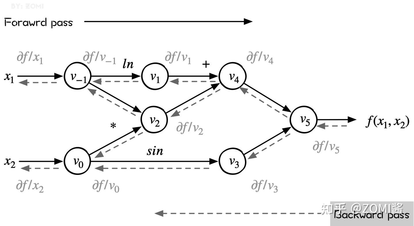
前向和后向兩種模式的過程表達如下,表的左列淺色為前向計算函數(shù)值的過程,與前向計算時相同,右面列深色為反向計算導數(shù)值的過程。
反向模式的計算過程如圖所示,其中:
viˉ=δyδvi
根據(jù)鏈式求導法則展開有:
?f?x=∑k=1N?f?vk?vk?x
可以看出,左側(cè)是源程序分解后得到的基本操作集合,而右側(cè)則是每一個基本操作根據(jù)已知的求導規(guī)則和鏈式法則由下至上計算的求導結(jié)果。
反向操作符重載實現(xiàn)
下面的代碼主要介紹反向模式自動微分的實現(xiàn)。目的是通過了解PyTorch的auto diff實現(xiàn),來了解到上面復雜的反向操作符重載實現(xiàn)自動微分的原理,值的主要的是千萬不要在乎這是 MindSpore 的實現(xiàn)還是 Tensorflow 版的實現(xiàn)(實際上都不是哈)。
首先,需要通過 typing 庫導入一些輔助函數(shù)。
from typing import List, NamedTuple, Callable, Dict, Optional

_name = 1
def fresh_name():
    global _name
    name = f'v{_name}'
    _name += 1
    return name
fresh_name 用于打印跟 tape 相關(guān)的變量,并用 _name 來記錄是第幾個變量。
為了能夠更好滴理解反向模式自動微分的實現(xiàn),實現(xiàn)代碼過程中不依賴PyTorch的autograd。代碼中添加了變量類 Variable 來跟蹤計算梯度,并添加了梯度函數(shù) grad() 來計算梯度。
對于標量損失l來說,程序中計算的每個張量 x 的值,都會計算值dl/dX。反向模式從 dl/dl=1 開始,使用偏導數(shù)和鏈式規(guī)則向后傳播導數(shù),例如:
dl/dx?dx/dy=dl/dy
下面就是具體的實現(xiàn)過程,首先我們所有的操作都是通過Python進行操作符重載的,而操作符重載,通過 Variable 來封裝跟蹤計算的 Tensor。每個變量都有一個全局唯一的名稱 fresh_name,因此可以在字典中跟蹤該變量的梯度。為了便于理解,__init__ 有時會提供此名稱作為參數(shù)。否則,每次都會生成一個新的臨時值。
為了適配上面圖中的簡單計算,這里面只提供了 乘、加、減、sin、log 五種計算方式。
class Variable:
    def __init__(self, value, name=None):
        self.value = value
        self.name = name or fresh_name()

    def __repr__(self):
        return repr(self.value)

    # We need to start with some tensors whose values were not computed
    # inside the autograd. This function constructs leaf nodes.
    @staticmethod
    def constant(value, name=None):
        var = Variable(value, name)
        print(f'{var.name} = {value}')
        return var

    # Multiplication of a Variable, tracking gradients
    def __mul__(self, other):
        return ops_mul(self, other)

    def __add__(self, other):
        return ops_add(self, other)

    def __sub__(self, other):
        return ops_sub(self, other)

    def sin(self):
        return ops_sin(self)

    def log(self):
        return ops_log(self)
接下來需要跟蹤 Variable 所有計算,以便向后應用鏈式規(guī)則。那么數(shù)據(jù)結(jié)構(gòu) Tape 有助于實現(xiàn)這一點。
class Tape(NamedTuple):
    inputs : List[str]
    outputs : List[str]
    # apply chain rule
    propagate : 'Callable[List[Variable], List[Variable]]'
輸入 inputs 和輸出 outputs 是原始計算的輸入和輸出變量的唯一名稱。反向傳播使用鏈式規(guī)則,將函數(shù)的輸出梯度傳播給輸入。其輸入為 dL/dOutputs,輸出為 dL/dinput。Tape只是一個記錄所有計算的累積 List 列表。
下面提供了一種重置 Tape 的方法 reset_tape,方便運行多次自動微分,每次自動微分過程都會產(chǎn)生 Tape List。
gradient_tape : List[Tape] = []

# reset tape
def reset_tape():
    global _name
    _name = 1
    gradient_tape.clear()
現(xiàn)在來看看具體運算操作符是如何定義的,以乘法為例子啦,首先需要計算正向結(jié)果并創(chuàng)建一個新變量來表示,也就是 x = Variable(self.value * other.value)。然后定義了反向傳播閉包 propagate,使用鏈規(guī)則來反向支撐梯度。
def ops_mul(self, other):
    # forward
    x = Variable(self.value * other.value)
    print(f'{x.name} = {self.name} * {other.name}')

    # backward
    def propagate(dl_doutputs):
        dl_dx, = dl_doutputs
        dx_dself = other # partial derivate of r = self*other
        dx_dother = self # partial derivate of r = self*other
        dl_dself = dl_dx * dx_dself
        dl_dother = dl_dx * dx_dother
        dl_dinputs = [dl_dself, dl_dother]
        return dl_dinputs

    # record the input and output of the op
    tape = Tape(inputs=[self.name, other.name], outputs=[x.name], propagate=propagate)
    gradient_tape.append(tape)
    return x
def ops_add(self, other):
    x = Variable(self.value + other.value)
    print(f'{x.name} = {self.name} + {other.name}')

    def propagate(dl_doutputs):
        dl_dx, = dl_doutputs
        dx_dself = Variable(1.)
        dx_dother = Variable(1.)
        dl_dself = dl_dx * dx_dself
        dl_dother = dl_dx * dx_dother
        return [dl_dself, dl_dother]

    # record the input and output of the op
    tape = Tape(inputs=[self.name, other.name], outputs=[x.name], propagate=propagate)
    gradient_tape.append(tape)
    return x

def ops_sub(self, other):
    x = Variable(self.value - other.value)
    print(f'{x.name} = {self.name} - {other.name}')

    def propagate(dl_doutputs):
        dl_dx, = dl_doutputs
        dx_dself = Variable(1.)
        dx_dother = Variable(-1.)
        dl_dself = dl_dx * dx_dself
        dl_dother = dl_dx * dx_dother
        return [dl_dself, dl_dother]

    # record the input and output of the op
    tape = Tape(inputs=[self.name, other.name], outputs=[x.name], propagate=propagate)
    gradient_tape.append(tape)
    return x

def ops_sin(self):
    x = Variable(np.sin(self.value))
    print(f'{x.name} = sin({self.name})')

    def propagate(dl_doutputs):
        dl_dx, = dl_doutputs
        dx_dself = Variable(np.cos(self.value))
        dl_dself = dl_dx * dx_dself
        return [dl_dself]

    # record the input and output of the op
    tape = Tape(inputs=[self.name], outputs=[x.name], propagate=propagate)
    gradient_tape.append(tape)
    return x

def ops_log(self):
    x = Variable(np.log(self.value))
    print(f'{x.name} = log({self.name})')

    def propagate(dl_doutputs):
        dl_dx, = dl_doutputs
        dx_dself = Variable(1 / self.value)
        dl_dself = dl_dx * dx_dself
        return [dl_dself]

    # record the input and output of the op
    tape = Tape(inputs=[self.name], outputs=[x.name], propagate=propagate)
    gradient_tape.append(tape)
    return x
grad 呢是將變量運算放在一起的梯度函數(shù),函數(shù)的輸入是 l 和對應的梯度結(jié)果 results。
def grad(l, results):
    dl_d = {} # map dL/dX for all values X
    dl_d[l.name] = Variable(1.)
    print("dl_d", dl_d)

    def gather_grad(entries):
        return [dl_d[entry] if entry in dl_d else None for entry in entries]

    for entry in reversed(gradient_tape):
        print(entry)
        dl_doutputs = gather_grad(entry.outputs)
        dl_dinputs = entry.propagate(dl_doutputs)

        for input, dl_dinput in zip(entry.inputs, dl_dinputs):
            if input not in dl_d:
                dl_d[input] = dl_dinput
            else:
                dl_d[input] += dl_dinput

    for name, value in dl_d.items():
        print(f'd{l.name}_d{name} = {value.name}')

    return gather_grad(result.name for result in results)
以公式5為例:
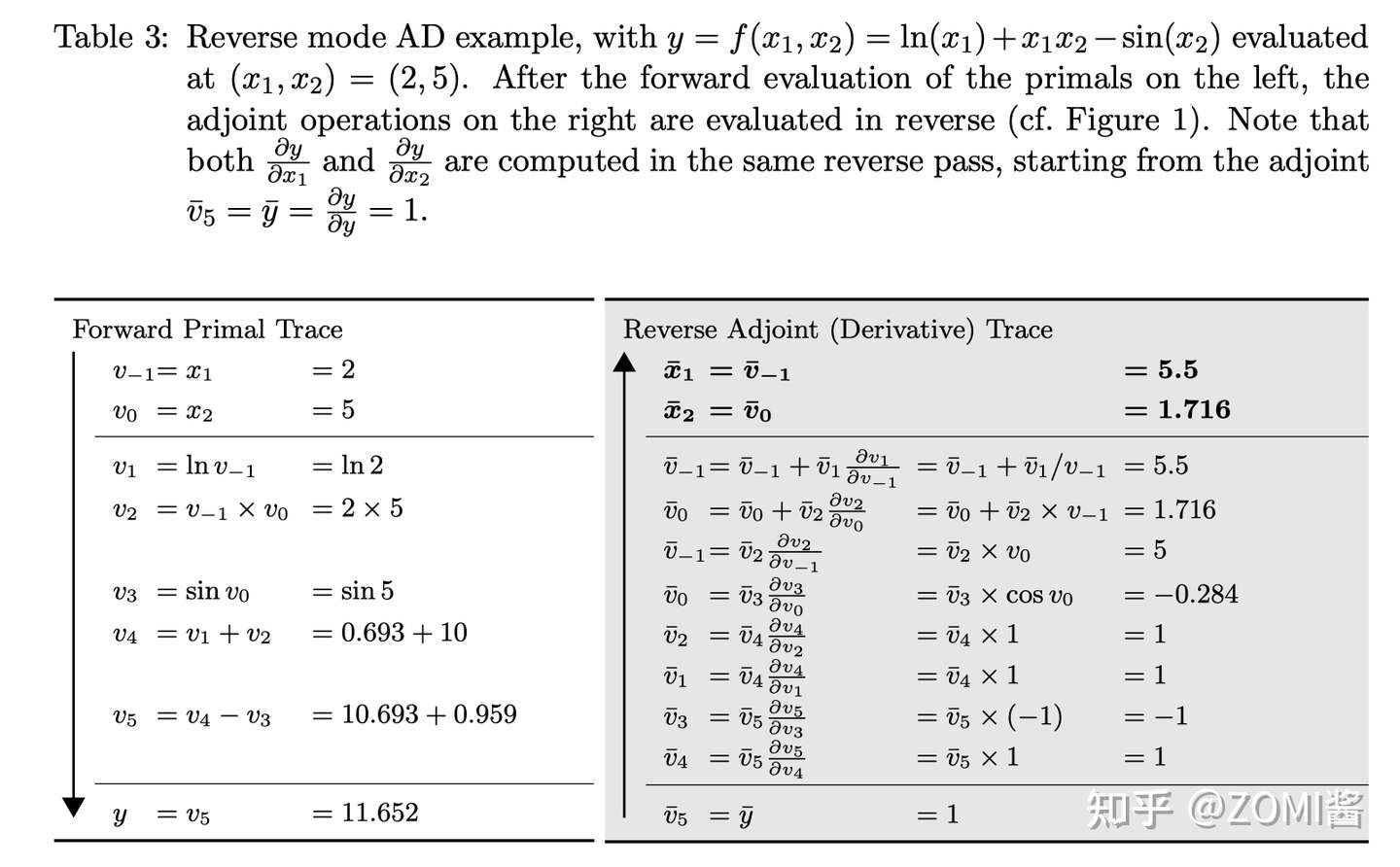
(1)f(x1,x2)=ln(x1)+x1x2?sin(x2)
因為是基于操作符重載OO的方式進行計算,因此在初始化自變量 x 和 y 的值需要使用變量 Variable 來初始化,然后通過代碼 f = Variable.log(x) + x * y - Variable.sin(y) 來實現(xiàn)。
reset_tape()

x = Variable.constant(2., name='v-1')
y = Variable.constant(5., name='v0')

f = Variable.log(x) + x * y - Variable.sin(y)
print(f)


v-1 = 2.0
v0 = 5.0
v1 = log(v-1)
v2 = v-1 * v0
v3 = v1 + v2
v4 = sin(v0)
v5 = v3 - v4
11.652071455223084
從 print(f) 可以看到是下面圖中的左邊正向運算,計算出前向的結(jié)果。下面的代碼 grad(f, [x, y]) 就是利用前向最終的結(jié)果,通過 Tape 一個個反向的求解。得到最后的結(jié)果啦。
dx, dy = grad(f, [x, y])
print("dx", dx)
print("dy", dy)


dl_d {'v5': 1.0}
Tape(inputs=['v3', 'v4'], outputs=['v5'], propagate=<function ops_sub.<locals>.propagate at 0x7fd7a2c8c0d0>)
v9 = v6 * v7
v10 = v6 * v8
Tape(inputs=['v0'], outputs=['v4'], propagate=<function ops_sin.<locals>.propagate at 0x7fd7a2c8c378>)
v12 = v10 * v11
Tape(inputs=['v1', 'v2'], outputs=['v3'], propagate=<function ops_add.<locals>.propagate at 0x7fd7a234e7b8>)
v15 = v9 * v13
v16 = v9 * v14
Tape(inputs=['v-1', 'v0'], outputs=['v2'], propagate=<function ops_mul.<locals>.propagate at 0x7fd7a3982ae8>)
v17 = v16 * v0
v18 = v16 * v-1
v19 = v12 + v18
Tape(inputs=['v-1'], outputs=['v1'], propagate=<function ops_log.<locals>.propagate at 0x7fd7a3982c80>)
v21 = v15 * v20
v22 = v17 + v21
dv5_dv5 = v6
dv5_dv3 = v9
dv5_dv4 = v10
dv5_dv0 = v19
dv5_dv1 = v15
dv5_dv2 = v16
dv5_dv-1 = v22
dx 5.5
dy 1.7163378145367738

 浙公網(wǎng)安備 33010602011771號